Separate events from periodic snapshots

An inventory movement records a change. An inventory snapshot records a balance at a particular boundary. Both can contain a warehouse, a product and a quantity, but their quantities answer different questions. Adding three closing balances does not tell you how many units were available at one time, and a missing snapshot does not mean that the warehouse was empty.

For an analyst or developer familiar with SQL aggregation, this distinction is a practical modeling decision. Use events to study activity during an interval and snapshots to study state at a boundary. The worked example keeps the two observations separate, checks snapshot coverage, and reconciles them only under explicit assumptions about the event stream and measurement scope.

Give events and snapshots different row definitions

The synthetic business has two warehouses, A and B, carrying the same product in identical physical units. A movement row represents one signed quantity change at a warehouse. A snapshot row represents that warehouse’s counted closing balance for one UTC reporting day. The source defines closing as the balance after all movements belonging to that day, immediately before the next day begins.

Microsoft’s fact-table guidance distinguishes transaction facts from periodic snapshots and uses daily inventory balances as a snapshot example. The useful distinction here is the observation, not the presence of a date column. Both tables have dates; one contains changes and the other contains states.

The fixture has three reporting days and a fixed, independently declared population of two warehouses. The example quantities and aggregates are small integers. The primary key on snapshots prevents two selected balances for the same warehouse and day, but it cannot require that every expected balance has arrived.

CREATE TEMP TABLE report_days (day TEXT PRIMARY KEY);
CREATE TEMP TABLE warehouses (warehouse TEXT PRIMARY KEY);
CREATE TEMP TABLE stock_snapshots (
  day TEXT NOT NULL,
  warehouse TEXT NOT NULL,
  units INTEGER NOT NULL,
  PRIMARY KEY (day, warehouse)
);
CREATE TEMP TABLE movements (
  movement_id INTEGER PRIMARY KEY,
  day TEXT NOT NULL,
  warehouse TEXT NOT NULL,
  delta_units INTEGER NOT NULL
);
INSERT INTO report_days VALUES ('2026-07-01'), ('2026-07-02'), ('2026-07-03');
INSERT INTO warehouses VALUES ('A'), ('B');
INSERT INTO stock_snapshots VALUES
  ('2026-07-01', 'A', 10), ('2026-07-01', 'B', 6),
  ('2026-07-02', 'A', 14), ('2026-07-02', 'B', 6),
  ('2026-07-03', 'A', 9);
INSERT INTO movements VALUES
  (1, '2026-07-02', 'A', 4),
  (2, '2026-07-03', 'A', -5),
  (3, '2026-07-03', 'B', 2);

CREATE TEMP VIEW daily_stock AS
SELECT d.day, COUNT(*) AS expected_warehouses,
       COUNT(s.warehouse) AS observed_warehouses,
       CASE WHEN COUNT(s.warehouse) = COUNT(*) THEN SUM(s.units) END
         AS network_units
FROM report_days d
CROSS JOIN warehouses w
LEFT JOIN stock_snapshots s ON s.day = d.day AND s.warehouse = w.warehouse
GROUP BY d.day;

SELECT * FROM daily_stock ORDER BY day;

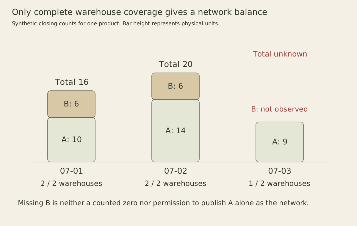
The first day has two expected and two observed warehouses, totaling 16 units. The second also has full coverage, totaling 20. The third has two expected but only one observed warehouse, so network_units is null. A’s nine units are known; the whole network’s balance is not established by these observations.

View full-size image ↗

Keep missing coverage in the reporting result

Summing only stored snapshots would report nine for July 3 and make the missing warehouse disappear. Filling B with zero would instead assert that B was counted and found empty. Neither follows from a row that failed to arrive. The expected warehouse population must come from the reporting contract, not from whichever rows happen to be present.

A real population can change when a warehouse opens, closes or leaves the reporting scope. Model those eligibility dates and build the expected set for each day. Do not infer closure from a missing extract. Conversely, do not require a snapshot before a warehouse becomes eligible. The fixed two-warehouse population is a deliberate simplification of this example.

The dbt data-test documentation describes assertions about uniqueness, nullness and relationships. A unique snapshot key is useful, but completeness requires comparison with an expected population. A relationship check should also reject snapshots or movements for undeclared warehouses instead of allowing them to vanish outside the report’s driving set.

Reconcile a change total with a balance boundary

The movement rows describe activity during July 2 and July 3. Their net change is four minus five plus two, or one unit:

SELECT day, SUM(delta_units) AS net_change
FROM movements
GROUP BY day
ORDER BY day;

SELECT SUM(delta_units) AS period_net_change
FROM movements
WHERE day >= '2026-07-02' AND day < '2026-07-04';

The daily changes are positive four and negative three; the period total is positive one. If the movement journal is complete, uses the same physical population, and includes every adjustment between the two closing boundaries, the July 1 closing balance of 16 implies a reconstructed July 3 balance of 17. That equation is a conditional reconciliation, not a replacement observation for the missing B snapshot.

Under those assumptions, A reconstructs as ten plus four minus five, or nine. B reconstructs as six plus two, or eight. This explains what to investigate when B’s final count is absent. It does not prove the journal was complete simply because its arithmetic produces a plausible balance. The absence of a B movement on July 2 means zero change only under a complete-journal contract.

View full-size image ↗

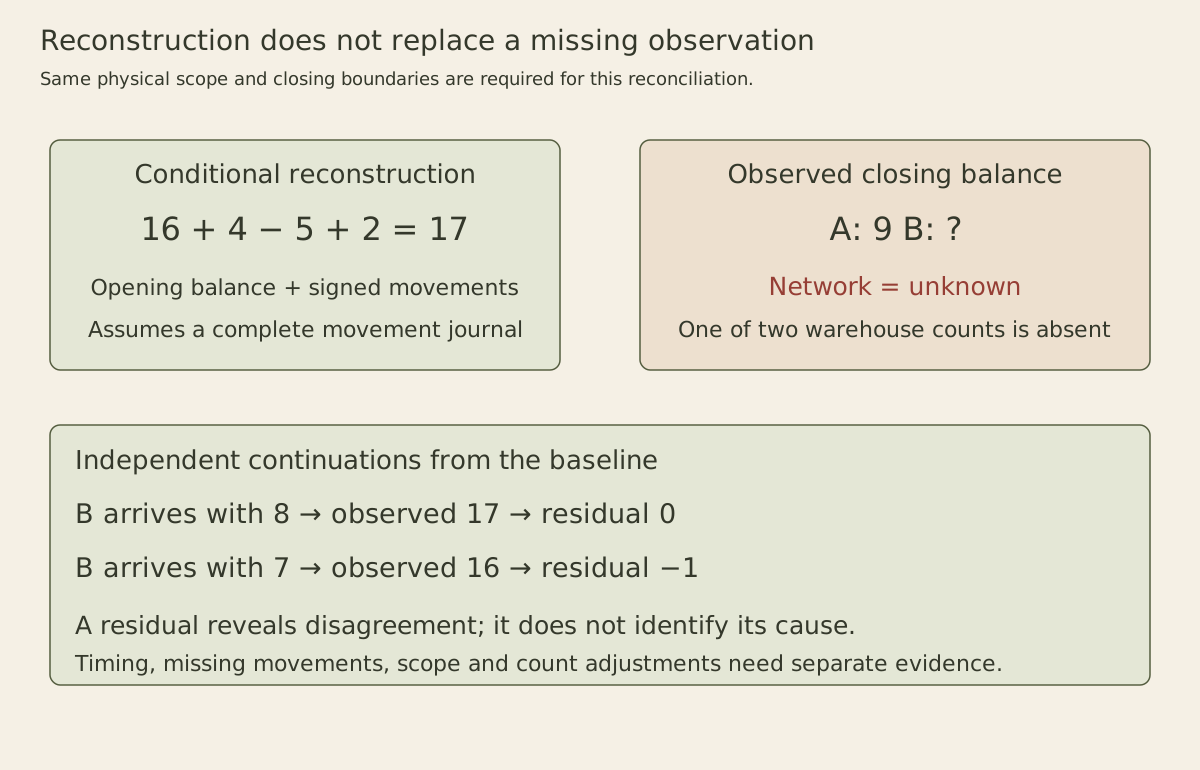
For a worked continuation, add B’s July 3 snapshot with eight units. The observed closing network balance becomes 17 and agrees with the reconstructed total. Add seven instead on a fresh baseline: the observed total becomes 16, leaving a reconciliation residual of negative one. Investigate timing, missing movements, scope differences or a stock-count adjustment. The residual alone cannot identify which explanation is true.

Decide whether time aggregation answers a real question

After adding B’s count of eight, the three daily closing balances are 16, 20 and 17. Their sum is 53. That is a sum across three stock observations, not 53 units simultaneously available and not a throughput measure. Taking the arithmetic mean yields 53 divided by three, about 17.67 units, interpreted specifically as the mean of those three daily closing observations.

It is not the continuously time-weighted average stock during the period. The snapshots contain no information about intraday peaks, shortages or the duration of intermediate balances. A business may reasonably use average closing stock, but the metric name should preserve that sampling convention.

This query only publishes that mean when all three expected days have complete warehouse coverage:

SELECT COUNT(*) AS expected_days,
       SUM(observed_warehouses = expected_warehouses) AS complete_days,
       CASE WHEN SUM(observed_warehouses = expected_warehouses) = COUNT(*)
            THEN AVG(network_units) END AS mean_daily_closing_units
FROM daily_stock;

On the original incomplete fixture it returns three expected days, two complete days and null mean. With B’s eight-unit snapshot added, it returns three, three and approximately 17.67. A plain AVG on the original view would skip the null day and return 18 from only 16 and 20. The PostgreSQL aggregate reference documents that aggregates such as AVG operate on non-null inputs; that behavior is not a missing-day policy.

Finally, keep warehouse transfers and stock ownership definitions consistent. A transfer can reduce one warehouse and increase another without changing network stock, but goods in transit need a declared place in the population. Two snapshots with different cutoff conventions can count the same goods twice or omit them. A shared product code and matching total are not enough to establish physical comparability.

Recreate the baseline for each exercise: add B with eight, add B with seven, and attempt a duplicate A snapshot for July 3. Check the observed total, reconciliation residual and primary-key rejection separately. Then remove a movement while keeping complete snapshots and explain why coverage can pass while reconciliation fails. The two tables complement each other because they preserve different evidence, rather than because either can automatically replace the other.