Read a tiny attention matrix without the mystique

For a student reading about transformers, attention becomes easier to inspect when you calculate one row yourself. Scaled dot-product attention turns query-key scores into weights, then uses those weights to combine value vectors. The weights determine a computation; they do not automatically explain why a model’s final answer is correct.

The Attention Is All You Need paper defines the operation as a softmax over scaled query-key products followed by multiplication by the value matrix. The example below uses deliberately chosen scores and two-dimensional values so every number can be checked by hand.

Begin after the score calculation

For one query and three keys, suppose the already-scaled scores are 0, ln(2), and ln(3). In a full attention layer, those scores would come from dot products divided by the square root of the key dimension. Choosing them directly here isolates the normalization step.

Softmax exponentiates each score and divides by the sum. The exponentials are 1, 2, and 3, so the weights are 1/6, 2/6, and 3/6. They are nonnegative and sum to one.

Let the value vectors be v1 = (1, 0), v2 = (0, 2), and v3 = (3, 1). The output is the weighted sum:

output = (1/6)*(1,0) + (2/6)*(0,2) + (3/6)*(3,1)
       = (1/6 + 9/6, 4/6 + 3/6)
       = (5/3, 7/6)

The largest attention weight belongs to the third value, but all three values contribute. A heat map showing only the weights would omit the vectors being combined. Different value vectors with the same weights can produce different outputs.

View full-size image ↗

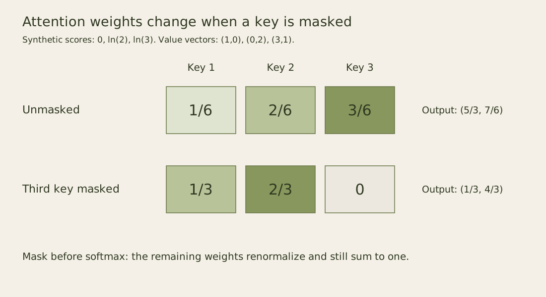
The figure shows one attention row, not an entire transformer. A full model has multiple positions, heads, layers, residual paths, and other operations. Keeping this example small prevents those details from hiding the basic weighted-sum calculation.

Apply a causal mask before softmax

Suppose the third key belongs to a future token that this query must not see. A causal mask excludes that position before normalization, commonly represented mathematically by replacing its score with negative infinity. Its exponential becomes zero.

The remaining unnormalized weights are 1 and 2. After renormalization, the weights become 1/3, 2/3, and 0. The output is now (1/3, 4/3). Simply setting the old third weight to zero would leave the weights summing to one half and would not perform the same attention operation.

In the transformer’s decoder, the mask prevents a position from using future output tokens during training. Without that restriction, the model could use information unavailable when generating the next token. The paper describes masking in its decoder attention, and the same causal idea underlies autoregressive generation.

A mask also needs correct indexing. A one-position shift can accidentally expose the next token or hide the current permitted context. Tests on tiny matrices are useful because you can identify exactly which positions should have zero weight.

Implement the arithmetic carefully

For numerical stability, subtract the maximum finite score before exponentiating. Softmax is unchanged by adding or subtracting the same constant from every score, while the subtraction reduces the chance of overflow. A production implementation also needs a defined behavior for an entirely masked row.

from math import exp, log

scores = [0.0, log(2), log(3)]
maximum = max(scores)
unnormalized = [exp(score - maximum) for score in scores]
weights = [value / sum(unnormalized) for value in unnormalized]
values = [(1, 0), (0, 2), (3, 1)]
output = [sum(w * value[j] for w, value in zip(weights, values))
          for j in range(2)]

This code demonstrates a single unmasked row. It is not a replacement for a tensor library’s batched attention implementation. When testing it, compare with the rational values above using a floating-point tolerance rather than exact equality.

Specify the mask’s shape before adding batches

For three positions in causal self-attention, a common allowed-position matrix is lower triangular. Query zero sees key zero. Query one sees keys zero and one. Query two sees all three. The diagonal is allowed because the hidden state at a position predicts the following token under the usual shifted-target training arrangement; allowing it does not reveal that next target.

View full-size image ↗

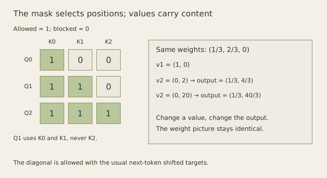
Write the expected allowed positions down before comparing libraries. Some APIs interpret a Boolean true as “keep,” while others use it to mark a blocked position. A mask can have the expected shape yet express the opposite policy. Padding masks introduce another constraint and should be combined with the causal rule deliberately.

Here is a scalar reference for the normalization step. It rejects an entirely excluded row, making the example’s policy explicit. A particular tensor backend may choose another documented behavior; match that contract when testing the real integration.

from math import exp, isclose, log

def masked_weights(scores, allowed):
    if len(scores) != len(allowed) or not any(allowed):
        raise ValueError("need matching lengths and an allowed key")
    maximum = max(score for score, keep in zip(scores, allowed) if keep)
    raw = [exp(score - maximum) if keep else 0.0
           for score, keep in zip(scores, allowed)]
    return [value / sum(raw) for value in raw]

weights = masked_weights([0.0, log(2), log(3)], [True, True, False])
assert isclose(weights[0], 1/3)
assert isclose(weights[1], 2/3)
assert weights[2] == 0.0

The reference assumes finite real scores at allowed positions. NaN and infinite values need separate input or numerical-failure handling. Add tests for a single allowed key, equal scores, a constant offset and a completely excluded row. These cases check specific invariants without requiring a GPU or a large model download.

Understand the scale factor

The division by the square root of the key dimension controls the size of query-key dot products. Under a simple assumption that components have roughly unit variance and contribute independently, the variance of a sum of component products grows with the dimension. Large scores can make softmax concentrate sharply, which affects its gradients during training. The scale factor addresses that magnitude effect; it does not normalize every learned query or guarantee a particular attention pattern.

Jay Alammar’s The Illustrated Transformer, published June 27, 2018, walks through learned query, key and value projections before the weighted sum. Its visual sequence helps connect these small numbers to the surrounding matrix operations. The numerical values and diagrams in this article are separate worked examples; no picture from that tutorial is reproduced here.

In the worked row, scaling has already happened before the chosen scores enter softmax. Dividing those same scores again would change the example. When reading an implementation, locate the scale operation and the mask explicitly so you know which matrix a visualization represents.

Keep interpretation claims narrow

Attention weights can help inspect a model computation, but a large weight on a token does not by itself prove that token caused the final decision in the way a reader imagines. The value projection, other heads, later layers, and residual connections also affect the output.

The paper Attention is not Explanation investigates limitations of treating attention distributions as explanations in its studied settings. It does not mean that attention visualizations are useless. It means that an explanation claim needs evidence beyond a visually appealing heat map.

For an application investigation, change a relevant input fact while preserving unrelated text and observe the output. You can also test whether removing or replacing a passage changes a decision. Such interventions answer a more concrete behavioral question than asking which token has the brightest color.

The small calculation gives you two checks to carry into larger models: masking happens before normalization, and weights only describe how the current value vectors are combined. When a diagram or explanation skips either point, return to the three-vector example and identify which part of the computation is missing.

For one final exercise, keep the masked weights fixed at one third and two thirds, but replace the second value with (0, 20). The second output coordinate becomes 40/3 instead of 4/3, while the displayed attention weights remain identical. This controlled change is enough to show why weights alone do not determine the represented content. It does not establish a universal interpretability result: it isolates one missing input to one attention calculation, which is exactly the boundary a useful explanation should state.