Choose AI mathematics from the next question

Choose the next mathematics topic from a question you need to answer about the system. If changing a vector’s length changes its retrieval rank, study the scoring operation. If a small evaluation has no errors, study what the sample can support. If an update makes a loss larger, study the step rule. Each question gives the abstraction somewhere concrete to attach.

I use this approach when planning a transition into AI engineering: write the observation, make the smallest numerical example that reproduces it, then identify the missing concept. This article assumes basic algebra and Python arithmetic. The examples are deliberately constructed calculations, not a trained model, an embedding benchmark or a production evaluation.

Ask why a similarity score changed

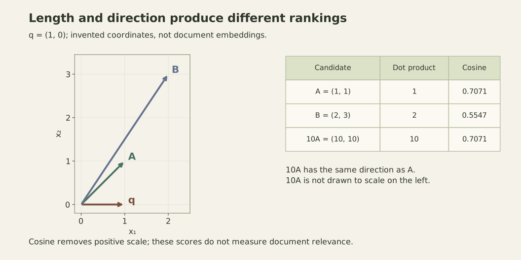
Suppose a query is represented by the two-dimensional vector q = (1, 0). Compare candidate A, (1, 1), with candidate B, (2, 3). Their coordinates are invented. They are not extracted from documents, so the calculation says nothing about which document a reader would find relevant.

The dot product multiplies matching coordinates and adds the results. With this query, A scores one and B scores two. A ranking based on the raw dot product puts B first. That result depends on both the vectors’ directions and their lengths.

Cosine similarity divides the dot product by the product of the two Euclidean lengths. The query has length one. A has length the square root of two; B has length the square root of thirteen. Their cosine scores are therefore about 0.7071 and 0.5547. Cosine puts A first because its direction is closer to the query direction.

The Stanford information-retrieval book’s dot-product section explains length normalization in a term-vector model. The same vector arithmetic explains our toy example. It does not establish that every embedding system should normalize, because the representation and intended scoring rule determine whether magnitude carries useful information.

from math import sqrt

q = (1, 0)
candidates = {"A": (1, 1), "B": (2, 3), "10A": (10, 10)}
for name, (x, y) in candidates.items():
    dot = q[0] * x + q[1] * y
    cosine = dot / sqrt(x * x + y * y)  # q has length 1
    print(name, dot, f"{cosine:.4f}")

Scaling A by ten raises its dot-product score from one to ten while preserving its cosine score. Positive scaling preserves direction; it does not preserve the raw dot product. A zero vector has no direction and makes the cosine denominator zero, so an implementation needs a defined policy for that case.

View full-size image ↗

The next study topics are vectors, dot products, norms and normalization. A useful stopping point for this learning session is being able to predict the effect of positive scaling and explain the zero-vector boundary. You can then inspect the actual retrieval system’s scoring contract. A cosine value is not automatically a calibrated probability that the result is correct.

Ask what zero observed errors means

Imagine twenty evaluation cases with no observed errors. The sample error fraction is zero. It does not follow that the system has zero error probability on future work, especially if the cases were selected because they were easy or copied from the same pattern.

For a small probability exercise, assume twenty independent trials with the same hypothetical error probability p. The probability of seeing no errors is (1 - p)^20: every trial must succeed. The NIST binomial-distribution reference gives the probability-mass function for a fixed trial probability; substituting zero counted errors produces this expression.

from fractions import Fraction

for p in (Fraction(1, 100), Fraction(1, 10), Fraction(1, 5)):
    no_errors = (1 - p) ** 20
    print(f"p={float(p):.2f}: P(no errors in 20)={float(no_errors):.6f}")

Even when the hypothetical error rate is ten percent, twenty error-free observations have probability about 0.1216 under these assumptions. The calculation shows that the observed result is possible under a substantially nonzero error rate. It does not say there is a 12.16 percent probability that the true rate is ten percent. Those conditionals run in different directions.

The next topics are random variables, independence, sampling and interval estimation. If you want a posterior probability about the error rate, you need an inferential model that supplies the missing assumptions; the forward binomial calculation alone is not one. If you want a confidence interval, choose and justify an interval procedure rather than treating the sample fraction as a certainty.

Also inspect how the cases were obtained. Twenty slight rewrites of one example may not behave like twenty independent trials. Repeated outputs from a fixed input answer another question from performance over varied user tasks. A good statistical formula cannot repair a sample that represents a different population from the one the product must serve.

For the immediate exercise, vary the trial count while keeping the assumed rate fixed. Explain why the probability of no errors falls as independent opportunities for an error accumulate. Then list which independence and sampling assumptions you would need to check before applying that reasoning to your own evaluation.

Ask why a downhill update increased the loss

Take the one-parameter loss L(w) = (w - 3)^2. Its minimum is at w = 3, and its derivative is 2(w - 3). Gradient descent updates the parameter by subtracting the derivative multiplied by a learning rate, eta:

w_next = w - eta * 2 * (w - 3).

At w = 0, the derivative is negative, so the update moves right toward the minimum. That direction does not make every step size safe. A sufficiently large step crosses the minimum and lands farther away on the other side.

3Blue1Brown’s October 2017 gradient-descent lesson explains cost functions, negative-gradient direction and the role of learning rate. The written lesson is by Grant Sanderson with a text adaptation by Josh Pullen. I use a separate one-variable quadratic here so the step-size behavior can be checked exactly; no neural network from the lesson was trained.

from fractions import Fraction

for eta in (Fraction(1, 4), Fraction(1), Fraction(11, 10)):
    w = Fraction(0)
    states = []
    for step in range(6):
        states.append((w, (w - 3) ** 2))
        w = w - eta * 2 * (w - 3)
    print("eta =", eta)
    print("w:", [float(value) for value, loss in states])
    print("loss:", [float(loss) for value, loss in states])

With a rate of one-quarter, the distance from three halves at each step. With a rate of one, the parameter alternates between zero and six, and the loss stays nine. With a rate of 1.1, the parameter crosses the minimum repeatedly while its distance grows by a factor of 1.2 per step. The update uses the correct derivative in all three cases.

View full-size image ↗

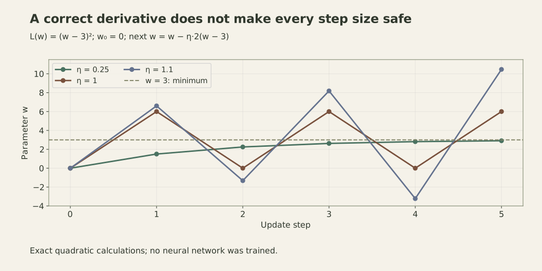
You can derive the boundary instead of guessing it. Let the error be e = w - 3. The update gives e_next = (1 - 2*eta) * e. For a nonzero starting error, its magnitude decreases when abs(1 - 2*eta) < 1, which here means 0 < eta < 1. That interval belongs to this particular quadratic and update rule. It is not a recommended learning-rate range for arbitrary neural networks.

The next topics are derivatives, gradients, local change and step-size stability. Multivariable losses add directions with different curvature; stochastic estimates add variation. Lower average training loss also does not prove that every example improved or that performance on unseen inputs improved. Keep the optimization target separate from the product outcome you eventually care about.

Turn the calculation into a learning decision

These three examples require different next steps. A changed similarity ranking calls for checking representation and normalization. An overconfident claim from a small sample calls for sampling and uncertainty. An unstable parameter update calls for understanding the loss and update dynamics. Starting a complete mathematics curriculum at random would make those distinctions harder to see.

Write one learning question in a form another engineer can check: “Does multiplying this vector by a positive constant preserve this score?” is more useful than “learn linear algebra.” Preserve the numerical example and your expected answer. When you can explain the result and the assumptions under which it holds, move to the next obstacle revealed by the real system.

This approach does not make broader foundations unnecessary. It gives the next study session a purpose and a stopping condition. The result should be a better engineering explanation, including where the calculation stops supporting the claim.