Insertion sort and almost-sorted input

Insertion sort is useful when a short array is already close to ordered because its work depends on the number of inversions. An inversion is a pair of positions whose values are in the wrong order: i < j but values[i] > values[j]. For a student who knows nested loops, counting those pairs explains why an algorithm with quadratic worst-case time can do little work on a particular input.

The word “almost” needs that definition. In [1, 2, 4, 3, 5], only the pair four and three is inverted. In [5, 4, 3, 2, 1], every earlier-later pair is inverted, giving ten inversions. Both arrays contain five distinct values, but insertion sort shifts one existing value in the first case and ten in the second.

Move one value into the sorted prefix

At iteration i, positions before i are already sorted. Save the current value, shift larger prefix values to the right, then place the saved value in the opening. The saved value must survive while its original slot is overwritten.

def insertion_sort(values):
    shifts = 0
    for i in range(1, len(values)):
        current = values[i]
        j = i
        while j > 0 and values[j - 1] > current:
            values[j] = values[j - 1]
            shifts += 1
            j -= 1
        values[j] = current
    return shifts

nearly = [1, 2, 4, 3, 5]
reversed_values = [5, 4, 3, 2, 1]
assert insertion_sort(nearly) == 1
assert insertion_sort(reversed_values) == 10
assert nearly == reversed_values == [1, 2, 3, 4, 5]

When three is inserted into [1, 2, 4], four shifts right once. Two is no larger than three, so shifting stops and three occupies the gap. The next value, five, already belongs after the sorted prefix and needs no shift.

The comparison uses > rather than >=. Equal values remain in their original order, which makes this version stable. If the elements are records, compare their sorting key while moving the complete record. Changing the condition to shift equal keys can change registration order or another meaningful order already present in the input.

View full-size image ↗

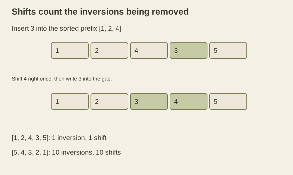
The diagram counts shifts of existing values. It does not count the final assignment of the saved value or every loop-condition check. A useful operation count needs that boundary stated before two implementations are compared.

Each shift removes one inversion

Consider the value currently being inserted. Every earlier value larger than it forms an inversion with it. The loop moves exactly those larger values past the current value, one position at a time. Earlier values no larger than it stay before it. Therefore the number of shifts in this iteration equals the number of inversions involving this value as the later element.

Every inversion has exactly one later element. Summing the shifts across iterations counts each original inversion once, so total shifts equal the original inversion count D. The prefix remains sorted because all values before the insertion position are no larger than the saved value and all values shifted after it are larger.

There is still work when D is zero. The outer loop visits every value, and most iterations make a comparison that determines no shift is needed. Total work is Θ(n + D), with Θ(n) on sorted input and Θ(n²) in the worst case. Princeton’s elementary-sorts material describes the same relation between insertion sort and inversions.

For distinct values in reverse order, D = n(n - 1) / 2, because every pair is inverted. Duplicate values do not count as inversions when equality is permitted in sorted order. An all-equal input therefore requires no shifts in the stable implementation.

A misplaced position count answers something else

The array [2, 3, 4, 5, 1] has every value away from its final position, yet it has only four inversions: each of two through five precedes one. Inserting the last value shifts four elements once. Counting “wrong positions” would describe this input as completely disordered and miss why insertion sort handles it cheaply.

A long reversed block inside an otherwise sorted array can have many inversions even if the rest of the data is untouched. If the reversed block has length k and its values stay between the surrounding values, that block alone contributes k(k - 1) / 2 inversions. The block’s length matters quadratically.

This is why a benchmark should name the input generator. A few random swaps, a short reversed run, and one value moved from the end to the front can produce different inversion counts. Calling all of them “nearly sorted” obscures the workload. Count shifts alongside time so that the observed work can be explained.

Keep the comparison with library sorting fair

The implementation uses constant additional storage beyond the input list and its loop variables. It also performs Python-level assignments, so timing it against a library sort mixes algorithm choice with interpreter overhead. The cost model assumes constant-time key comparisons; a key that parses a document or performs network access invalidates that simplified model.

Production sorting libraries can exploit structure too. Python’s sorting HOWTO notes that its sorting algorithm can use existing order. A result showing that insertion sort benefits from low inversion count does not establish that it beats the standard sort on a given application.

For a controlled exercise, enumerate short arrays with repeated values, compute their inversion count using a simple pair loop, and compare it with the instrumented shift count. Keep that quadratic counting routine outside performance measurements. The test should verify both the sorted result and the equality between shifts and inversions; either one alone misses part of the explanation.

Binary insertion separates comparisons from moves

A binary search can locate the gap within the sorted prefix. It cannot create that gap in a packed array: the intervening records still need to move. This distinction matters when comparing keys is expensive but moving a reference is cheap. Count both operations before deciding whether the change helps.

For stability, search for the first prefix key strictly greater than the saved key. That places the new record after existing equal keys. A lower-bound search would place it before those records and reverse their arrival order across repeated insertions.

def binary_insertion_sort(records, key):
    comparisons = shifts = 0
    for i in range(1, len(records)):
        current = records[i]
        current_key = key(current)
        lo, hi = 0, i
        while lo < hi:
            middle = (lo + hi) // 2
            comparisons += 1
            if key(records[middle]) <= current_key:
                lo = middle + 1
            else:
                hi = middle
        for j in range(i, lo, -1):
            records[j] = records[j - 1]
            shifts += 1
        records[lo] = current
    return comparisons, shifts

backwards = list(range(8, 0, -1))
ordered = list(range(1, 9))
assert binary_insertion_sort(backwards, key=lambda x: x) == (17, 28)
assert binary_insertion_sort(ordered, key=lambda x: x) == (13, 0)
assert backwards == ordered

registrations = [(2, 'Zoe'), (1, 'Ava'), (2, 'Amy')]
binary_insertion_sort(registrations, key=lambda record: record[0])
assert registrations == [(1, 'Ava'), (2, 'Zoe'), (2, 'Amy')]

On eight distinct values in reverse order, ordinary insertion sort performs twenty-eight key comparisons and twenty-eight shifts. The binary version makes seventeen key comparisons but still twenty-eight shifts. On an already sorted list of eight values, ordinary insertion sort makes seven key comparisons and no shifts; this binary version makes thirteen comparisons and no shifts. Binary search improves one input’s comparison count while worsening the other’s.

View full-size image ↗

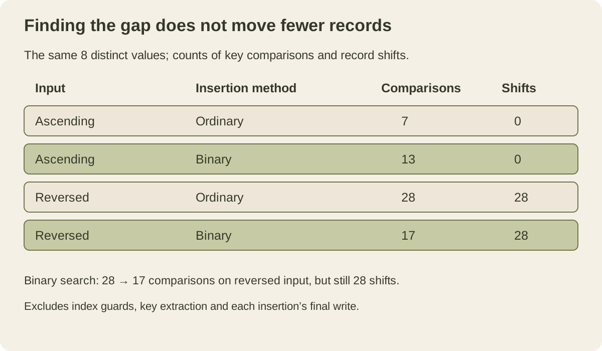
Here a key comparison means comparing two data keys. The counts exclude index-bound checks, calls to the key function, and the final write of each saved record. The binary version evaluates the saved key once per insertion but can recompute keys in the prefix. It therefore is not a promise of one key extraction per input record. A separate cached-key array can provide that property at the cost of extra storage and synchronized moves.

Binary insertion reduces worst-case key comparisons to O(n log n), but its worst-case time remains quadratic because it shifts every inversion. Its time is O(n log n + D) under the same constant-cost model. A preliminary check against the last prefix key could skip the search when the record already belongs at the end; that is a different implementation with different counts.

As an exercise, add a comparison counter to the original function without counting a failed index guard as a key comparison. Reproduce the four columns in the figure, then enumerate short inputs with duplicate keys and tagged records. Both implementations should make the same number of shifts, produce sorted keys, and preserve the tag order within each equal-key group. This checks the cost explanation and the stability contract together.