Sorting lower bounds with a decision tree

Any deterministic algorithm that sorts distinct keys using only pairwise comparisons needs Ω(n log n) comparisons in the worst case. A decision tree explains the bound by counting how many input orders the algorithm must distinguish. For a student learning lower bounds, three labeled items are enough to see the whole argument before introducing factorials.

Assume all keys are distinct and that a comparison asks a binary question such as whether A is smaller than B. Arithmetic on key digits, array indexing by key value, and assumptions that the input is already nearly sorted are outside this model. A lower bound is useful only when its permitted operations and input family are clear.

Every comparison chooses a branch

Imagine running a fixed sorting algorithm but leaving the comparison results undecided. Its first comparison forms the tree’s root. One branch represents true and the other false. The algorithm may choose different next comparisons on those branches, producing a tree whose leaves represent completed decisions.

Three labeled items A, B, and C can appear in six strict relative orders. A correct sorter must distinguish all six because each order requires a different permutation of the original positions. If two incompatible orders reached the same leaf, the algorithm would produce the same position permutation for both and fail on at least one.

A binary tree of height two has at most four leaves. It cannot distinguish six possible orders. Height three can have up to eight leaves, so some input requires at least three comparisons. That does not say every input must require three; shorter paths can finish after two.

View full-size image ↗

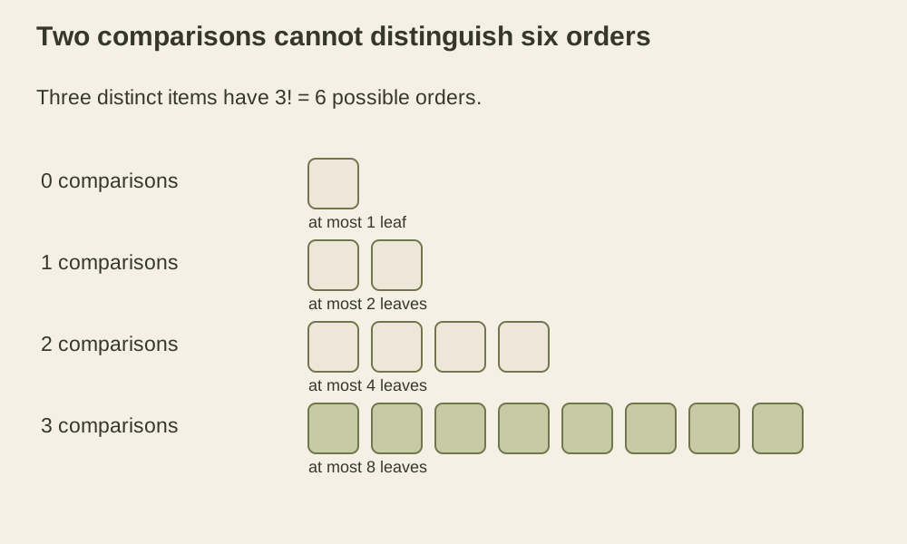
The picture shows the capacity argument, not a claim that every full tree corresponds to a valid sorting algorithm. Counting leaves supplies a necessary condition. Constructing an algorithm that reaches a particular bound is a separate task.

Generalize six orders to n factorial

For n distinct labeled items, there are n! relative orders. A binary decision tree with maximum depth h has at most 2^h leaves. Correctness therefore requires 2^h >= n!, which gives h >= ceil(log2(n!)).

To see the growth without using a detailed approximation, take even n. The largest n/2 factors of n! are each at least n/2, so n! >= (n/2)^(n/2). Taking logarithms gives a lower bound of (n/2) * log2(n/2), which is Ω(n log n). Odd sizes follow by reducing to the adjacent smaller even size.

An O(n log n) comparison sort matches that asymptotic worst-case lower bound. It does not follow that every such implementation has the same exact comparison count, memory use, stability, or runtime. Princeton’s mergesort discussion includes comparison lower bounds alongside the upper-bound analysis.

Inspect comparison paths on all small permutations

An instrumented insertion sort illustrates the difference between a worst-case lower bound and the count for an individual input. For three distinct keys, the code performs two comparisons on some permutations and three on the rest.

from itertools import permutations


def insertion_comparisons(source):
    original = list(source)
    values = original.copy()
    count = 0
    for i in range(1, len(values)):
        current = values[i]
        j = i
        while j > 0:
            count += 1
            if values[j - 1] <= current:
                break
            values[j] = values[j - 1]
            j -= 1
        values[j] = current
    assert values == sorted(original)
    return count

counts = [insertion_comparisons(order) for order in permutations(range(3))]
assert counts.count(2) == 2
assert counts.count(3) == 4
assert max(counts) == 3
assert insertion_comparisons(iter([3, 1, 2])) == 3

The helper consumes its input once and retains the original values for its final reference check, so a one-use iterator works too. The counter covers only comparisons in the insertion loop; copying and the separate reference sort are verification work outside that counter.

The average count over these six equally likely inputs is 16 / 6, or about 2.67. That average is above log2(6), about 2.58, as the information argument suggests. Extending a worst-case statement to an average-case statement requires a distribution over inputs; uniform permutations is a specific choice, not an automatic property of production data.

Randomization also needs a precise claim. Random choices can improve a bad deterministic pivot policy’s expected behavior, but they do not make arbitrary comparison sorting require sublinear-in-n log n expected work for every possible input distribution. The deterministic tree argument is the starting point; proving a randomized lower bound requires accounting for the algorithm’s distribution over such trees.

Identify when the leaf count changes

Repeated keys reduce the number of distinct sorted-value arrangements that must be distinguished. If multiplicities are fixed at m1, m2, ..., the number of distinct value permutations is n! / (m1! * m2! * ...). An all-equal input contains far less ordering information than a permutation of distinct values. Algorithms can exploit that difference when their comparison and output contracts permit it.

A promise that the input belongs to a restricted family changes the counting argument too. Sorting a sequence known to have only a few inversions is a smaller problem than accepting every permutation. The general worst-case lower bound does not forbid faster behavior on that restricted family.

Counting sort and radix sort inspect bounded keys or digits and use them to select buckets. Their operation model supplies information beyond a binary comparison of complete keys. Their linear bounds under suitable key-domain assumptions therefore do not contradict the comparison lower bound. Princeton’s sorting applications places these algorithm choices in the context of key types and application requirements.

For a new sorting claim, write down the key domain, allowed operations, whether equal records must stay stable, and which cost is being bounded. Then ask how many outcomes the algorithm has to distinguish. That is a more precise way to evaluate a “faster than n log n” claim than applying the familiar bound without its assumptions.

Construct one complete three-item tree

A concrete tree shows why a short path and a long path can both belong to a correct sorter. First compare A with B. If A is smaller, compare B with C: a true result finishes at A, B, C after two comparisons. A false result leaves C’s position relative to A undecided, so one more comparison chooses A, C, B or C, A, B. The other branch is symmetric after exchanging A and B’s roles.

def order_three(values):
    if len(values) != 3:
        raise ValueError('exactly three distinct comparable keys are required')
    trace = []

    def before(i, j):
        outcome = values[i] < values[j]
        trace.append((i, j, outcome))
        return outcome

    if before(0, 1):
        if before(1, 2):
            order = (0, 1, 2)
        elif before(0, 2):
            order = (0, 2, 1)
        else:
            order = (2, 0, 1)
    else:
        if before(0, 2):
            order = (1, 0, 2)
        elif before(1, 2):
            order = (1, 2, 0)
        else:
            order = (2, 1, 0)
    return order, trace

order, trace = order_three([30, 10, 20])
assert order == (1, 2, 0)
assert trace == [(0, 1, False), (0, 2, False), (1, 2, True)]
for values in permutations(range(3)):
    order, trace = order_three(values)
    assert [values[i] for i in order] == sorted(values)
    assert len(trace) in (2, 3)

The returned tuple is a permutation of input positions. It is not a new set of numeric values and does not depend on labels being alphabetically sortable. The input must already satisfy the distinct, consistently comparable key contract; the length check does not validate that semantic precondition. This keeps the example inside the stated comparison model instead of quietly classifying values through another operation.

View full-size image ↗

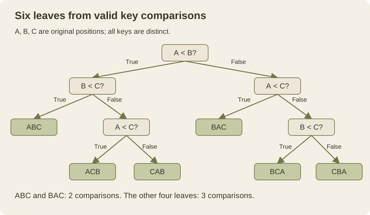
There are six leaves, with two at depth two and four at depth three. The leaf labels are strict orders of the original items. Some branches end early because the comparisons already imply the missing relation by transitivity. For example, A smaller than B and B smaller than C imply A smaller than C without a third query. The eight-leaf capacity of a full height-three binary tree is not a requirement to keep asking questions after the answer is known.

This tree achieves the three-comparison worst-case bound for three distinct items. It does not establish that the simple ceiling of the information bound is attainable for every larger input size. A tree of abstract yes/no questions also has more freedom than a tree whose questions must be valid comparisons of available keys. Necessary leaf capacity and a realizable sorting strategy are separate obligations.

The same tree has different averages under different input distributions. Suppose, as a hypothetical workload, ABC and BAC each occur with probability 0.4 and each other order occurs with probability 0.05. Eighty percent of cases then use two comparisons and twenty percent use three, giving 0.8*2 + 0.2*3 = 2.2 comparisons on average. Its worst case is still three. These probabilities describe an example distribution, not measurements of a real application.

As an exercise, assign all probability to one three-comparison leaf, then compare the new average with the uniform average. Next, enumerate the three-item tree and verify that no two different strict orders reach the same leaf. This separates two questions often mixed in performance claims: whether every allowed input can be sorted correctly, and how often a particular workload follows each valid path.