Distinguish event time from processing time
Assign six delayed observations to two sets of five-minute windows, then test replay, timestamp offsets, exact boundaries and a clock-disagreement counterexample.
A phone records a tap while it is offline and uploads it after reconnecting. A chart of taps during the user’s morning should usually place that tap at its reported occurrence time. A chart of work handled by the ingestion operator should place it when that operator processed the record. Both charts can be correct while showing different counts in the same five-minute interval.
This article is for a developer or data engineer learning streaming terminology. You need basic SQL grouping and an understanding of UTC offsets. We will assign six constructed observations to windows with SQLite 3.45.1, then inspect a hypothetical replay and a suspicious clock reading. These are executed SQL examples over toy timestamps, not a running Beam or Flink pipeline, a device trace or a measured network experiment.
Name the clock and the boundary
Event time refers to when an event occurred at its source. In a data pipeline, the system commonly represents it with a timestamp carried by the record. Processing time comes from the clock of the machine executing a particular operation. The Flink time concepts describe both and explain why processing-time behavior depends on arrival speed, operator progress and outages.
That operation matters. A broker receiving a message, an application handler starting work and a downstream aggregate processing it are different boundaries. A field named received_at is not automatically the processing time of every later operator. Our processed_at means the time at one stipulated processing boundary. It is supplied as toy data so the assignment can be inspected without waiting for a live clock.
The event field is named reported_event_at deliberately. A device timestamp is a claim about occurrence time; its presence does not establish that the device clock was accurate. Preserve the distinction between the time represented by a field and the evidence that supports it. That distinction becomes visible in the final counterexample.
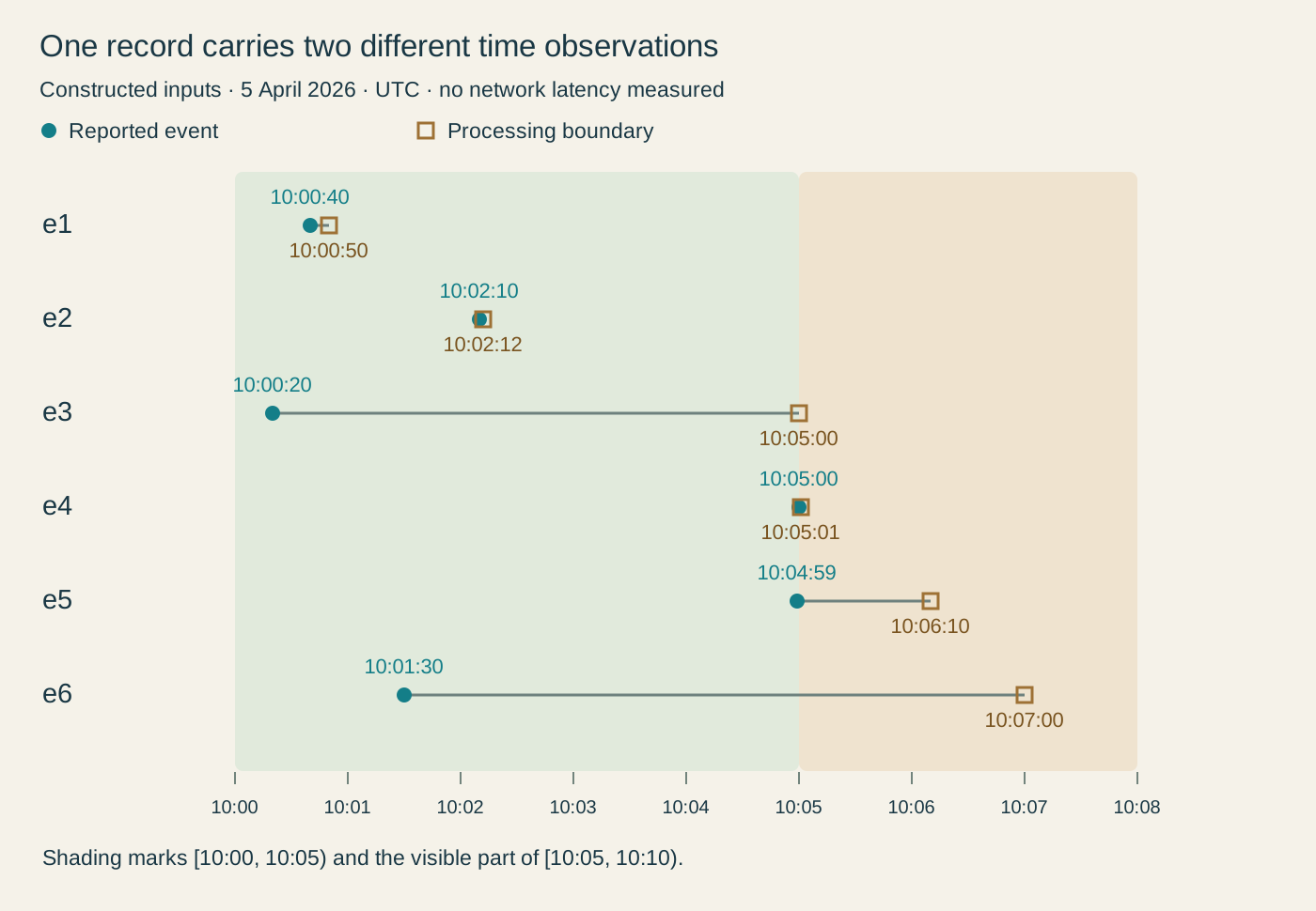
The dots are supplied timestamps. Connecting them shows their difference; it is not a measured breakdown of network, queue or execution latency.
Normalize instants before comparing them
Run the five SQL blocks in order in one new SQLite database. Each event identifier appears once. The examples use positive Unix seconds, whole-second timestamps and fixed five-minute UTC windows anchored to the Unix epoch. They do not implement local calendar days, daylight-saving rules, fractional-second policy or duplicate-delivery handling.
CREATE TABLE observations (
  event_id TEXT PRIMARY KEY,
  reported_event_at TEXT NOT NULL,
  processed_at TEXT NOT NULL
);
INSERT INTO observations VALUES
 ('e1', '2026-04-05T10:00:40Z',      '2026-04-05T10:00:50Z'),
 ('e2', '2026-04-05T10:02:10Z',      '2026-04-05T10:02:12Z'),
 ('e3', '2026-04-05T10:00:20Z',      '2026-04-05T10:05:00Z'),
 ('e4', '2026-04-05T10:05:00Z',      '2026-04-05T10:05:01Z'),
 ('e5', '2026-04-05T17:04:59+07:00', '2026-04-05T10:06:10Z'),
 ('e6', '2026-04-05T10:01:30Z',      '2026-04-05T10:07:00Z');
CREATE VIEW normalized AS
SELECT event_id, unixepoch(reported_event_at) AS event_s,
       unixepoch(processed_at) AS processing_s
FROM observations;
SELECT COUNT(*) AS unparseable_rows FROM normalized
WHERE event_s IS NULL OR processing_s IS NULL;
The first result is zero unparseable rows. SQLite’s date and time documentation defines unixepoch as seconds since 1970-01-01 00:00:00 UTC and explains how explicit offsets are converted. The +07:00 value for e5 therefore represents 10:04:59 UTC, not 17:04:59 UTC. Comparing the raw text strings as local clock labels would misplace that observation.
The parse check only establishes that these six supplied values produced numbers. It is not a production timestamp validator, nor evidence that a device reported the correct instant. A real contract should define accepted syntax, precision, offset requirements and what happens when a record cannot be interpreted. Silently dropping failed conversions would change the population before you even compare clocks.
Follow one delayed observation through both assignments
For the nonnegative integer seconds in this fixture, integer division by 300 selects a five-minute bucket; multiplying by 300 returns its start. Each interval includes its start and excludes its end. Thus 10:04:59 belongs to the interval beginning at 10:00, while exactly 10:05:00 belongs to the next interval.
SELECT event_id,
       datetime(event_s, 'unixepoch') AS reported_event_utc,
       datetime(processing_s, 'unixepoch') AS processing_utc,
       processing_s - event_s AS apparent_gap_s,
       time((event_s / 300) * 300, 'unixepoch') AS event_window,
       time((processing_s / 300) * 300, 'unixepoch') AS processing_window
FROM normalized
ORDER BY processing_s, event_id;
Read e3 closely. Its reported event time is 10:00:20, but its stipulated processing time is 10:05:00. It contributes to the 10:00 event-time window and the 10:05 processing-time window. The computed difference is 280 seconds. The row is compatible with an offline upload, but the two timestamps alone do not prove that explanation or identify how much time was spent offline, in transit or waiting in a queue.
e4 makes the boundary explicit: its event time is exactly 10:05:00, so both assignments use the later window. e6 arrives after the others at this processing boundary even though its reported occurrence precedes e2. Sorting by processing time is therefore not the same as sorting by event time. The Beam programming guide explicitly notes that records need not appear in the order in which their events were generated.
The displayed window columns contain only time-of-day to keep this one-day table short. The grouped query below retains the full date. A production key must not accidentally combine 10:00 on different days just because a chart label omitted the date.
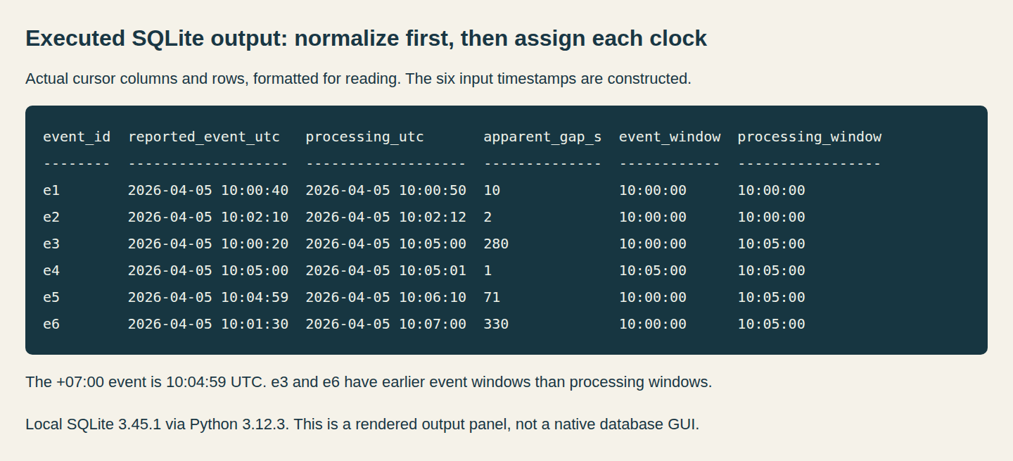
This reading panel is a real browser capture of recorded SQLite output. The query ran locally; the six input timestamps remain constructed examples.
Ask the question before choosing the count
The next query creates one membership per event for each clock and groups the memberships separately. UNION ALL retains both analytical views; it does not mean that twelve distinct user events occurred.
WITH memberships AS (
  SELECT 'event' AS clock, event_id, (event_s / 300) * 300 AS start_s
  FROM normalized
  UNION ALL
  SELECT 'processing', event_id, (processing_s / 300) * 300
  FROM normalized
)
SELECT clock, datetime(start_s, 'unixepoch') AS window_start_utc,
       COUNT(*) AS events
FROM memberships
GROUP BY clock, start_s
ORDER BY clock, start_s;
By event time, the counts are five in the 10:00 window and one in the 10:05 window. By processing time, they are two and four. Both views account for all six event identifiers. Their disagreement is about interval ownership, not a lost row or a different total population.
Choose the first view for a question such as “When did these reported user actions happen?” Choose the second for “When did this operator handle these records?” A capacity investigation may need the second boundary even when a user-activity report uses the first. Document the clock in the metric name or definition rather than calling both outputs simply “events per five minutes.”
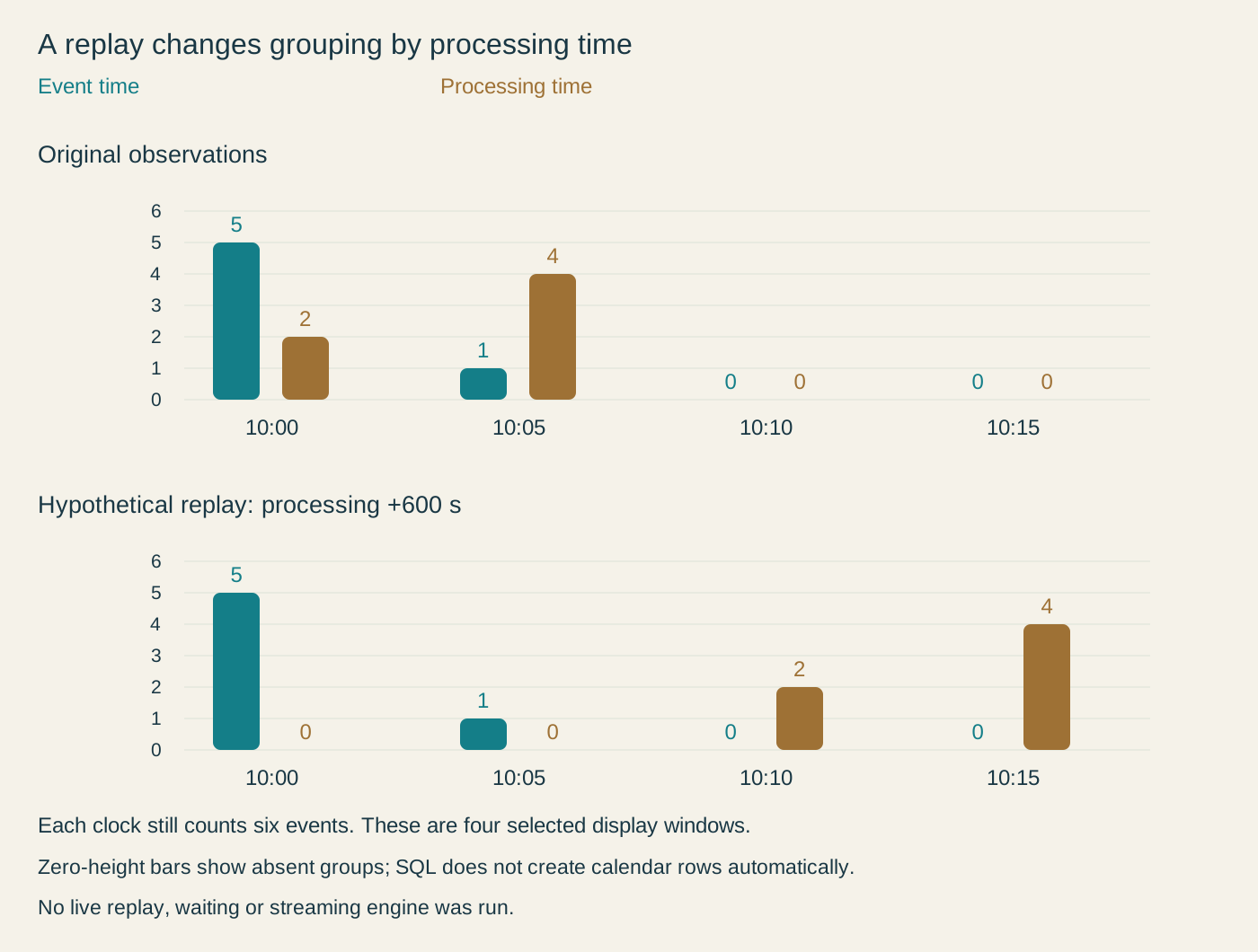
Each view counts six rows. The hypothetical replay changes processing-window ownership while preserving the reported event timestamps.
Reprocessing changes one clock, not necessarily the other
The replay query adds 600 seconds to every processing timestamp while retaining the reported event timestamp. It is a constructed alternative schedule, not an actual ten-minute wait or a live replay service.
WITH replay AS (
  SELECT event_id, event_s, processing_s + 600 AS processing_s
  FROM normalized
), memberships AS (
  SELECT 'event' AS clock, event_id, (event_s / 300) * 300 AS start_s
  FROM replay
  UNION ALL
  SELECT 'processing', event_id, (processing_s / 300) * 300
  FROM replay
)
SELECT clock, datetime(start_s, 'unixepoch') AS window_start_utc,
       COUNT(*) AS events
FROM memberships
GROUP BY clock, start_s
ORDER BY clock, start_s;
The event-time counts remain five and one in their original windows. The processing-time counts move to 10:10 and 10:15, still two and four. That is useful for understanding reproducibility: the original occurrence labels can survive a different processing schedule, while processing-time membership follows the new schedule.
This stability has conditions. We retained the same six records, identifiers, event timestamps and assignment rule. Changing the event-time extraction, losing a record, counting a delivery twice or applying a different retention policy can change the result. Flink’s discussion explicitly qualifies its consistent event-time result with all data having arrived. Selecting an event timestamp alone does not supply completeness, deduplication or a finalization policy.
If a replay preserves an old stored processed_at column, that column describes the earlier processing observation. It is not the replay operator’s current clock merely because the replay reads it. Keep original observations and new attempt observations named separately when both are needed.
Window ownership is different from knowing the final answer
At the toy processing cutoff of 10:03, only two recorded events contribute to the 10:00 event window. After all six rows have been observed, five contribute. The assignment rule has stayed the same; the available evidence has grown.
SELECT 'first observation' AS view_name, COUNT(*) AS event_window_count
FROM normalized
WHERE event_s >= unixepoch('2026-04-05T10:00:00Z')
  AND event_s < unixepoch('2026-04-05T10:05:00Z')
  AND processing_s <= unixepoch('2026-04-05T10:03:00Z')
UNION ALL
SELECT 'all six recorded events', COUNT(*)
FROM normalized
WHERE event_s >= unixepoch('2026-04-05T10:00:00Z')
  AND event_s < unixepoch('2026-04-05T10:05:00Z');

WITH suspect(event_s, processing_s) AS (
 VALUES (unixepoch('2026-04-05T10:10:00Z'),
         unixepoch('2026-04-05T10:06:00Z'))
)
SELECT processing_s - event_s AS apparent_gap_s,
       time((event_s / 300) * 300, 'unixepoch') AS event_window,
       time((processing_s / 300) * 300, 'unixepoch') AS processing_window
FROM suspect;
The first query returns two and five. It does not establish that five is the final total of a real unbounded stream. Our finite fixture ends at six supplied records; a running system needs a separate policy for progress, delayed records and result updates. Those decisions cannot be inferred from the five-minute bucket expression.
The final query introduces one separate suspicious observation. Its reported event time is 10:10, while its processing time is 10:06. Subtraction returns minus 240 seconds, and the two windows differ. This does not demonstrate negative network latency. A fast source clock, an inaccurate processing clock or a bad timestamp transformation could produce such a record. The pair alone cannot identify which explanation is correct.
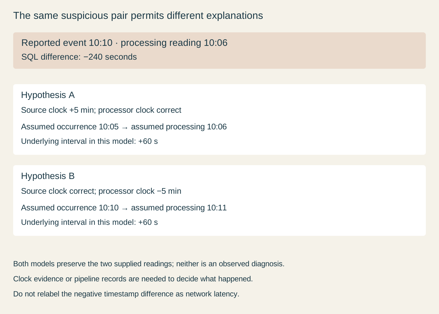
Alternative explanations are hypotheses, not measured diagnoses. Keep the original values and obtain additional clock or pipeline evidence before correcting them.
Clamping the negative difference to zero would make a dashboard look cleaner while hiding the disagreement. Replacing the event timestamp with processing time would change the question and move interval membership. A useful operational response is to flag the record under a declared timestamp-quality policy, retain its original fields and investigate with additional evidence. This article does not implement that policy.
Check the boundary with a small mutation
Change only e3’s processing timestamp to 10:04:59 in a fresh copy of the fixture. Its event-time membership must stay in the 10:00 window, while its processing membership moves from the later window to the earlier one. Processing counts become three and three; event counts remain five and one.
Next change e5 from 17:04:59+07:00 to the equivalent 10:04:59Z spelling. Every normalized value and count should remain unchanged. Finally, move e4’s reported event timestamp back one second without changing its processing timestamp. The event-time counts become six in the earlier window and no row for the empty later window. The query reports observed groups; it does not automatically generate zero-count calendar rows.
These mutations test three different decisions: which clock defines ownership, whether offsets describe the same instant, and which side owns an exact boundary. Once those are explicit, an event-time report and an operational processing-time report can coexist without silently answering each other’s questions.