Counting missing values without changing the denominator
Count rows, submissions and observed ratings correctly with runnable SQL, an invitation denominator, empty cohorts and explicit missingness rules.
COUNT(*) counts rows. COUNT(rating) counts rows whose rating is not null. That difference decides whether an unanswered survey question stays in your response-rate denominator. A zero rating is an answer and belongs in both counts; an unknown rating belongs only in the row count.
If you are learning SQL for analytics, start by naming the population you want to measure. “Average rating” usually means the average among people who supplied a rating. “Rating response rate” asks how many eligible people supplied one. Those measures can use the same table and still need different denominators.
Four rows, three answers
This toy survey has four recorded participants. Ratings use a scale from zero through five. Participant 103 skipped the question, so the database stores null. Participant 104 chose zero deliberately.
CREATE TEMP TABLE survey (
  participant_id INTEGER PRIMARY KEY,
  rating INTEGER
);
INSERT INTO survey VALUES (101, 5), (102, 4), (103, NULL), (104, 0);

SELECT
  COUNT(*) AS participants,
  COUNT(rating) AS answered,
  COUNT(*) - COUNT(rating) AS unanswered,
  AVG(rating) AS mean_answered,
  1.0 * COUNT(rating) / NULLIF(COUNT(*), 0) AS response_rate
FROM survey;
The query returns four participants, three answers, one unanswered question, a mean of 3.0, and a response rate of 0.75. These statements were checked with SQLite 3.45.1. The distinction between counting rows and counting non-null expressions also appears in the PostgreSQL aggregate documentation.
The multiplier of 1.0 asks SQLite to perform a fractional division. Without it, dividing two integers can truncate a response rate. The null guard on the denominator also documents what should happen when the table contains no participants: the rate is undefined. A reporting layer can display that state as “no eligible participants.” Calling it zero would assert that a population existed and nobody answered.
The average is nine divided by three. Including zero is necessary because zero is part of the declared rating scale. Replacing null with zero before averaging would instead produce nine divided by four, or 2.25. That operation adds an answer which the participant never supplied.
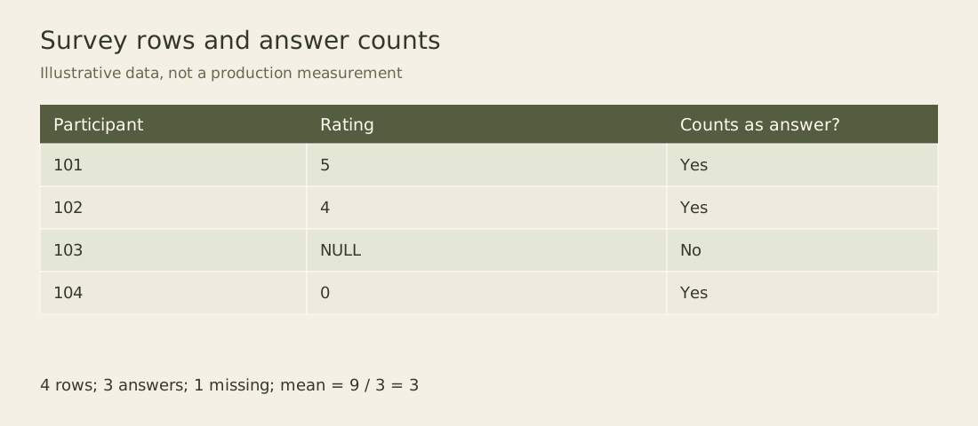
The two counters share their input rows. Only the rule for including a rating differs. A useful dashboard shows the response count next to the mean so readers can see how much observed evidence supports that mean.
Filtering changes the population
Suppose you move the missing-value condition into a filter:
SELECT COUNT(*) AS remaining_rows, AVG(rating) AS mean_answered
FROM survey
WHERE rating IS NOT NULL;
This returns three rows and the same mean of 3.0. The average did not change because it already ignored null ratings. The row count did change. If you compute a response rate after that filter using answered rows divided by remaining rows, every included row has answered and the result becomes 100 percent.
A filter is appropriate when your stated population is respondents to that question. It is inappropriate when your denominator is all eligible participants. Read the report label aloud before accepting the query. “Share of recorded participants who rated” and “share of ratings that are non-null” describe different calculations even though their SQL differs by one condition.
The same issue appears in product telemetry. A table containing only emitted events cannot count users whose devices failed to emit an event. The denominator needs an independent eligibility table if the metric refers to all invited or active users. Missing rows and null fields are separate forms of absence.
Count conditions without losing other rows
You can count several answer groups in one aggregation while preserving the original population:
SELECT
  SUM(CASE WHEN rating >= 4 THEN 1 ELSE 0 END) AS high_ratings,
  SUM(CASE WHEN rating = 0 THEN 1 ELSE 0 END) AS zero_ratings,
  SUM(CASE WHEN rating IS NULL THEN 1 ELSE 0 END) AS missing_ratings
FROM survey;
The result is two high ratings, one zero rating, and one missing rating. Here the case expression returns an explicit zero for a row outside the requested group. That makes the counting rule easy to inspect. Be careful with COUNT(CASE WHEN condition THEN 1 ELSE 0 END): both one and zero are non-null, so it counts every row.
For a table with no rows, these sums return null in SQLite. If your reporting contract defines each empty-group count as zero, apply the default to the final aggregate. Applying defaults to individual measurements has a different meaning, as the altered average demonstrated.
Start from invitations when submissions can be absent
The four-row example assumes every eligible participant already has a row. Many real survey pipelines store only submitted forms. In that design, COUNT(*) on the submissions table cannot reveal how many invited people never opened the form. You need a separate invitation population, defined at the same reporting cutoff as the submissions.
The next fixture distinguishes four cases: two observed ratings, an unanswered question inside a submitted form, a person with no submitted form, and a cohort with no invitations. It also includes a cohort whose submitted ratings are all null. The cohort names are arbitrary labels, and every person here is eligible for the question. This is synthetic data, not a measured response pattern.
CREATE TEMP TABLE cohorts (cohort TEXT PRIMARY KEY);
CREATE TEMP TABLE invitations (
  participant_id INTEGER PRIMARY KEY,
  cohort TEXT NOT NULL
);
CREATE TEMP TABLE submissions (
  participant_id INTEGER PRIMARY KEY,
  rating INTEGER CHECK (rating BETWEEN 0 AND 5)
);
INSERT INTO cohorts VALUES ('north'), ('south'), ('followup'), ('empty');
INSERT INTO invitations VALUES
  (101, 'north'), (102, 'north'),
  (103, 'south'), (104, 'south'), (105, 'south'),
  (106, 'followup'), (107, 'followup');
INSERT INTO submissions VALUES
  (101, 5), (102, 4), (103, NULL), (104, 0),
  (106, NULL), (107, NULL);

SELECT c.cohort,
  COUNT(i.participant_id) AS invited,
  COUNT(s.participant_id) AS submitted,
  COUNT(s.rating) AS rated,
  AVG(s.rating) AS mean_rating,
  1.0 * COUNT(s.rating)
    / NULLIF(COUNT(i.participant_id), 0) AS rating_coverage
FROM cohorts AS c
LEFT JOIN invitations AS i ON i.cohort = c.cohort
LEFT JOIN submissions AS s ON s.participant_id = i.participant_id
GROUP BY c.cohort
ORDER BY c.cohort;
The checked results are:
| Cohort | Invited | Submitted | Rated | Mean rating | Rating coverage |
|---|---|---|---|---|---|
| empty | 0 | 0 | 0 | NULL | NULL |
| followup | 2 | 2 | 0 | NULL | 0 |
| north | 2 | 2 | 2 | 4.5 | 1 |
| south | 3 | 2 | 1 | 0 | 1/3 |
The empty cohort still produces a null-extended row because the query begins with cohorts. Therefore COUNT(*) would report one row for that cohort, even though nobody was invited. Counting the non-null primary key from invitations gives the intended zero. The same reasoning explains why COUNT(s.participant_id) measures submitted forms while COUNT(s.rating) measures supplied ratings.
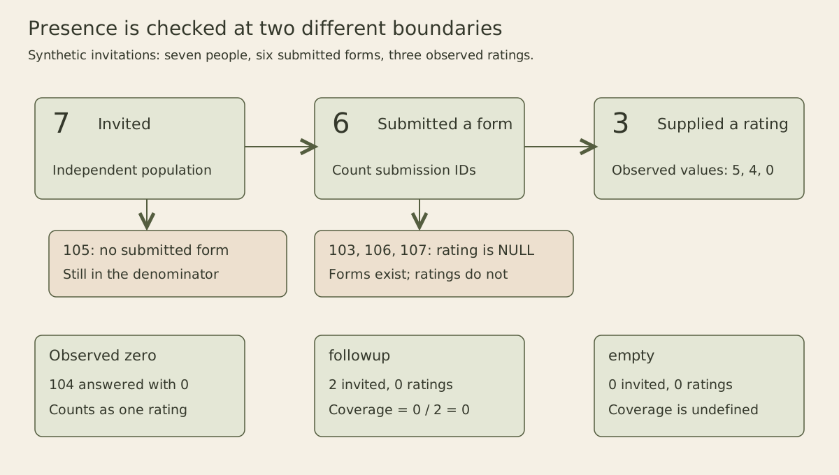
The figure follows presence at two boundaries. A missing submission and a null question value both reduce rating coverage, but they point to different follow-up work. One might require checking invitation delivery; the other might require investigating the question design or its import rules. SQL alone cannot select the explanation.
The primary key on submissions.participant_id makes the one-submission assumption enforceable. If the product allows revisions, first select one authorized revision per participant under an explicit time and status rule. Otherwise, a participant with three submissions can enlarge both counts and disguise a missing participant elsewhere. Counting distinct invitation IDs repairs only that one denominator; it does not automatically repair a mean that still includes repeated ratings.
For followup, zero coverage means an eligible population exists and no rating was observed. For empty, the rate is undefined because no eligible population exists. For south, the mean of zero is a real observed score from participant 104; it is not a display default. Preserve all three meanings when sending data to a chart or API. A numeric zero plus an observation count of one tells a different story from a null mean plus an observation count of zero.
A useful implementation choice is to expose numerator and denominator alongside the rate, rather than storing only a rounded percentage. A client can display “1 of 3” and choose an appropriate number of decimal places. The query result for one third is a floating-point approximation, so reporting 33.3% is a presentation decision, not greater measurement precision.
The outer-join counting pitfall is also discussed in Lukas Eder’s jOOQ article on COUNT. Its performance comparisons concern particular systems and versions. The transferable point here is the expression’s nullability; this article makes no claim that one spelling is faster on your workload.
Test the report as a population calculation
A small mutation exercise is more informative than checking only the first happy-path result. Add a submission (105, 2). South should still have three invitees, but its submitted count rises to three, rated count rises to two, mean becomes one, and coverage becomes two thirds. Next change participant 104’s rating from zero to null. The invitation count must remain three; the mean becomes two because only participant 105 now supplies a rating. Start with a fresh copy of the fixture, apply these two mutations in order on that same copy, then recreate the baseline before repeating the exercise.
If those changes alter the number of invitees, the query is mixing population selection with answer availability. If the count of rated people exceeds invitees, inspect duplicate submissions or eligibility joins before capping the percentage in the dashboard. A capped percentage hides a broken relationship while leaving the mean and subgroup comparisons wrong.
Missingness still needs an explanation
SQL can identify nulls without explaining why they occurred. A skipped question, a parsing failure, a privacy deletion, and a field absent in an older schema might all arrive as null. If those reasons matter to interpretation, preserve a separate reason column or an ingestion audit record.
This distinction matters especially when comparing groups. A mean calculated from a handful of willing respondents may not represent everyone invited. Counting non-null values correctly establishes the observed sample size; it does not establish that the sample is representative. Imputation requires a separate statistical argument and should remain visible in the dataset and report.
Before using the example on a larger survey, test an all-null group and an empty group. The all-null group has participants but no observed mean; the empty group has no participants at all. Keep those outcomes separate in your chart labels. That small distinction stops a missing measurement from becoming an invented zero and stops an absent population from becoming a misleading response rate.