Count the critical path in a ripple-carry adder
Calculate propagation through a four-bit ripple-carry adder using explicit hypothetical gate delays, then connect the result to a register timing budget.
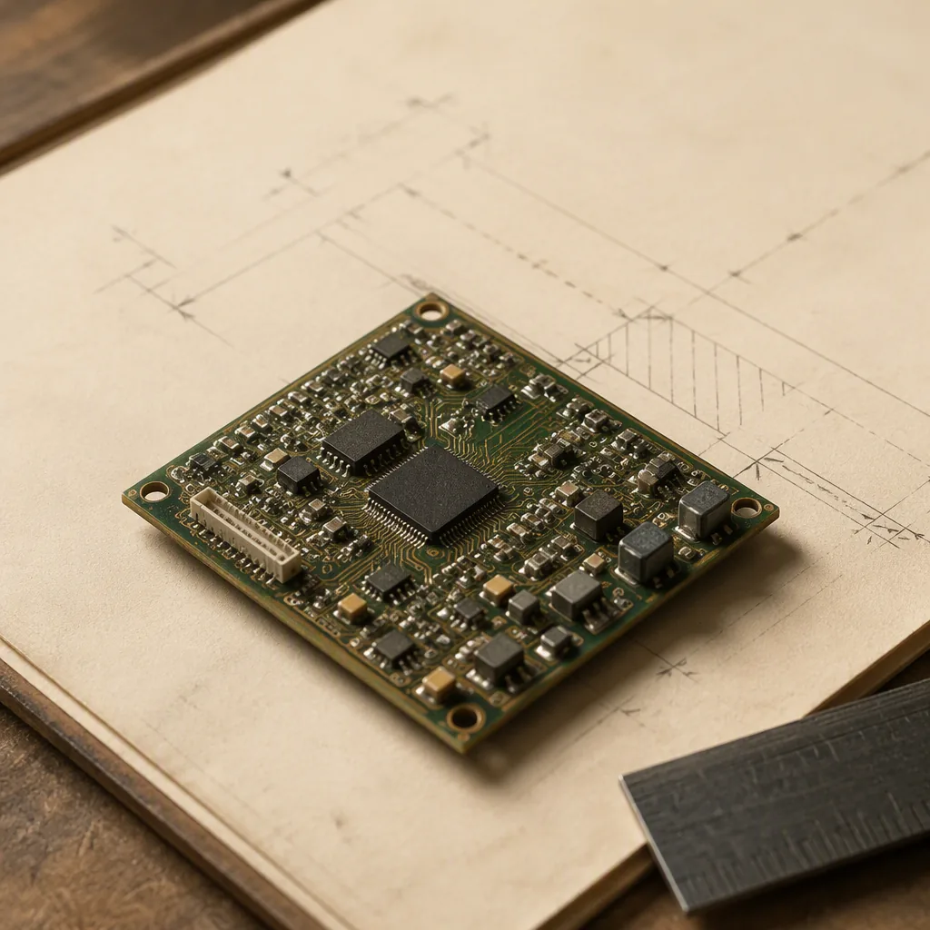
A ripple-carry adder waits for a carry to travel through successive bit positions. Its longest relevant path can therefore grow with the word width, even though the programmer sees one addition instruction. For a student connecting Boolean logic to processor timing, a four-bit example makes that delay visible without pretending to describe a particular chip.
All delays below are hypothetical. They are bounds assigned to a simple gate model, not measurements from a board or a commercial standard-cell library. Real delay depends on the selected cells, their input transitions, output loads, wiring, voltage, and temperature.
Give each full adder a contract
At bit position i, a full adder receives operand bits A and B and an incoming carry. It produces a sum bit and an outgoing carry. Define the propagate signal as P = A XOR B and the generate signal as G = A AND B. The outgoing carry is G OR (P AND carry_in), while the sum is P XOR carry_in.
Use the following simplified timing assumptions. Each XOR has a maximum delay of two nanoseconds. Each AND or OR has a maximum delay of one nanosecond. Both operands and the initial carry become valid at time zero. Ignore wires in this model and allow every gate to compute concurrently once its inputs are valid.
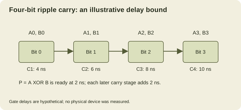
The propagate signals become valid at two nanoseconds. The generate signals become valid at one nanosecond. For the first outgoing carry, the propagate-and-carry term settles at three nanoseconds, and the final OR settles at four. Later stages receive their incoming carry after their local propagate signal is already available.
| Signal | Latest valid time in the model |
|---|---|
| P at every bit | 2 ns |
| Carry into bit 1 | 4 ns |
| Carry into bit 2 | 6 ns |
| Carry into bit 3 | 8 ns |
| Carry out of bit 3 | 10 ns |
| Sum bit 0 | 4 ns |
| Sum bit 3 | 10 ns |
This calculation uses the rule that a gate’s output becomes valid after its last relevant input is valid plus the gate’s propagation bound. The digital abstraction notes derive path-based maximum delay reasoning for combinational circuits.
Trace a carry-producing input
Consider 0111 + 0001. At bit zero, adding one and one generates a carry. Bits one and two each contain one operand bit set and the other cleared, so they propagate that carry. The result is 1000.
The arithmetic is immediate when written on paper. The circuit still needs signals to settle. Intermediate outputs can temporarily reflect old carries or old operands. Sampling a sum before the propagation contract has elapsed can observe a transient value, even though the stable Boolean function is correct.
A path bound also needs interpretation. The ten-nanosecond calculation is a conservative bound for this specific network and delay model. It is not proof that every addition takes exactly ten nanoseconds to settle, or that every structural path is sensitized by every input transition. Static timing analysis deliberately provides guarantees across allowed conditions instead of guessing from a favorable example.
You can reproduce the bound with a small recurrence. Let carry_time start at zero. For each bit, calculate sum_time = max(2, carry_time) + 2, then calculate the next carry as max(1, max(2, carry_time) + 1) + 1. The four sum times are 4, 6, 8, and 10 nanoseconds; the outgoing carry times are the same sequence.
Recalculate when an input arrives late
The recurrence should describe input arrival times rather than assume every input is equally early. For each bit, form propagate and generate after the later operand arrives. Then wait for the later input at each carry or sum gate. This is an arrival-time calculation, not a simulation of the intermediate binary waveform.
def ripple_bounds(a_times, b_times, carry_time=0):
    if not a_times or len(a_times) != len(b_times):
        raise ValueError("operand timing lists must have equal nonzero width")
    sums, carries = [], []
    for a_time, b_time in zip(a_times, b_times):
        operand_time = max(a_time, b_time)
        propagate = operand_time + 2
        generate = operand_time + 1
        sums.append(max(propagate, carry_time) + 2)
        carry_time = max(generate, max(propagate, carry_time) + 1) + 1
        carries.append(carry_time)
    return sums, carries

assert ripple_bounds([0]*4, [0]*4) == ([4, 6, 8, 10], [4, 6, 8, 10])
assert ripple_bounds([0]*4, [0]*4, 3) == ([5, 7, 9, 11], [5, 7, 9, 11])
assert ripple_bounds([0, 0, 0, 9], [0]*4) == ([4, 6, 8, 13], [4, 6, 8, 13])
print("3 arrival-time cases passed")
In the second case, the initial carry becomes valid at three nanoseconds. The first carry output moves from four to five, rather than shifting by the full three nanoseconds, because the original calculation was already waiting two nanoseconds for propagate. The remaining ripple stages inherit the extra one-nanosecond delay.
In the third case, only operand A’s highest bit is late, arriving at nine nanoseconds. Its propagate signal becomes valid at eleven and its generate signal at ten. Carry into that bit is already valid at eight, so the operand path determines both the final sum and carry bound of thirteen nanoseconds. Counting carry stages alone would miss this late-input condition.
For N bits with all inputs valid at zero, the recurrence gives a final bound of 2*N + 2 nanoseconds in this particular gate model. The first stage costs four and each later stage adds two. That formula is not a device-independent law: dedicated carry cells and different decompositions have different timing arcs. It is a compact consequence of assumptions that you can check and change.
Put registers around the adder
A synchronous datapath usually has a launching register before the combinational logic and a capturing register after it. The clock period must allow clock-to-output delay from the first register, the adder’s maximum path delay, and setup time at the second register. Clock skew and uncertainty alter that budget.
For an illustrative zero-skew path, suppose the launch register needs one nanosecond to produce a valid output and the destination needs one nanosecond of setup time. A ten-nanosecond adder then requires a period of at least twelve nanoseconds in the idealized model. Taking the reciprocal gives about 83.3 MHz. That is an arithmetic consequence of the assigned numbers, not a performance prediction for manufactured hardware.
The sequential logic chapter explains why maximum combinational delay appears in the setup constraint. Minimum delay matters separately for hold time. Making an adder faster can improve setup margin while making a short path elsewhere harder to hold.
Choose a different carry organization
A carry-lookahead or prefix structure computes carry information with more parallelism. It can shorten the logic depth of wide additions, but it uses additional gates and wiring. Physical placement becomes significant as signals span larger regions. Comparing only the number of Boolean levels leaves out fanout and wire delay.
A ripple chain can still be sensible for a small datapath or a design whose timing budget is loose. FPGA devices also provide dedicated carry resources, so a gate-by-gate model may poorly predict their implementation. The synthesis and timing tools must evaluate the architecture available on the chosen device.
Pipelining is another option, but it changes when the result arrives and how carries cross stage boundaries. A cut through the middle of an adder requires storing the intermediate carry and aligning the remaining operand bits. Registering arbitrary signals without preserving those relationships changes the computation.
A pipeline cut must preserve the input pair
Split the four-bit adder after the low two bits. The first stage calculates the low two sum bits and carry C2. The pipeline register must keep C2 together with the original upper halves of A and B and the low sum. The second stage adds the upper halves and that saved carry, while forwarding the matching low sum to the final output register.
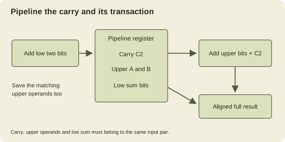
The two-bit combinational bound is six nanoseconds under the original assumptions. Adding the one-nanosecond clock-to-Q and one-nanosecond setup budget gives an illustrative period of eight nanoseconds per stage. A fully occupied pipeline can then accept one input pair every eight nanoseconds, compared with twelve for the single-stage design. The result takes two cycles, or sixteen nanoseconds, to travel from the initial launch to final capture. The throughput improves while the individual transaction latency grows.
This comparison assumes zero skew, no stalls, aligned control signals and no extra path dominating either stage. Pipeline registers add area, clock load and power. Short bypass paths, including the saved low sum, still need hold checks. The frequency arithmetic alone does not show that the physical design satisfies those requirements.
A useful functional check represents the registered bundle explicitly. It can prove the arithmetic alignment for every four-bit input pair without pretending to verify the eight-nanosecond clock claim.
def stage_one(a, b):
    low = (a & 3) + (b & 3)
    return low & 3, low >> 2, a >> 2, b >> 2

def stage_two(bundle):
    low_sum, carry, upper_a, upper_b = bundle
    upper_sum = upper_a + upper_b + carry
    return (upper_sum << 2) | low_sum

for a in range(16):
    for b in range(16):
        assert stage_two(stage_one(a, b)) == a + b
print("256 aligned input pairs passed")
The result includes the fifth carry bit, so the comparison covers sums up to thirty. If stage two accidentally uses the next transaction’s upper operands, even correct adders produce a wrong answer. For example, the first transaction 3 + 1 needs saved carry one and upper halves zero. Combining that carry with upper halves from a following 12 + 0 transaction produces sixteen instead of four. A valid bit or transaction tag must travel with the bundle when bubbles or stalls are introduced.
For a further exercise, feed a sequence of different input pairs through a one-entry bundle register and compare the delayed outputs against a queue of expected sums. Include a bubble and state whether it advances or holds each stage. This tests the scheduling rule that a pure addition truth table cannot capture.
For software performance work, the lesson is narrow and useful: one source-level addition does not imply one generic gate delay. Instruction latency, throughput, and the processor’s clock period depend on different aspects of the implementation. A small ripple chain supplies a concrete example of why those quantities need separate definitions.