Check a gradient with finite differences before trusting training

A gradient check compares a derivative with changes in the scalar function it is supposed to differentiate. For a custom loss or backward pass, that comparison can expose a sign, reduction or indexing error before training. Passing it establishes agreement only at the tested inputs and numerical resolution.

If you know partial derivatives and basic Python, this foundation lesson gives you a small check with an exact answer, then deliberately breaks its assumptions. We will distinguish truncation, floating-point loss of information, an uninformative direction and a nondifferentiable point. Every dataset and function below is a constructed example; no neural network training result is claimed.

Start with an answer that does not depend on floating point

Consider f(x,y) = x³ + 3xy + 2y². At (1,-2), the function equals three and its gradient is (-3,-5):

g_x = 3x² + 3y
g_y = 3x + 4y
D_h(v) = [f(p + h v) - f(p - h v)] / (2h)

For the x coordinate, expand the cubic on both sides. The even powers of the perturbation cancel. The result is exactly g_x + h²; for the y coordinate, it is exactly g_y. The corresponding forward x difference has error 3xh + h². These are algebraic identities for this polynomial, not estimates of rounding behavior.

Run the four Python blocks in order in one session. Fraction makes the first comparison exact; it is a teaching tool rather than a suggested numeric representation for a large model.

from fractions import Fraction as Q


def f(x, y):
    return x**3 + 3*x*y + 2*y*y


def central(fun, point, direction, h):
    plus = tuple(z + h*d for z, d in zip(point, direction))
    minus = tuple(z - h*d for z, d in zip(point, direction))
    return (fun(*plus) - fun(*minus)) / (2*h)


point = (Q(1), Q(-2))
gradient = (Q(-3), Q(-5))
for h in (Q(1, 10), Q(1, 100), Q(1, 1000)):
    dx = central(f, point, (1, 0), h)
    dy = central(f, point, (0, 1), h)
    assert dx == gradient[0] + h*h
    assert dy == gradient[1]
    print(h, dx, dy)

The x estimates are −2.99, −2.9999 and −2.999999; every y estimate is −5. Under sufficient smoothness, Taylor expansion gives central differences an error of order h², compared with the usual order h for forward differences. The leading term can vanish, as it does for the quadratic y dependence here. Do not infer an identical error constant for every parameter.

PyTorch’s gradcheck mechanics describes reconstructing a real-valued function’s Jacobian by perturbing inputs and comparing it with automatic differentiation. This lesson implements only scalar directional differences. It does not execute PyTorch or cover complex derivatives.

View full-size image ↗

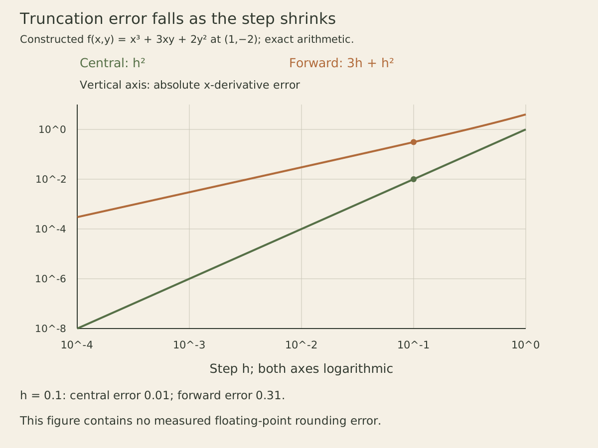
The plotted curves contain exact polynomial errors. They deliberately do not invent a measured rounding-error curve or imply that ever-smaller floating-point steps keep improving a check.

A harmless constant can destroy the numerical signal

Adding a constant leaves the mathematical derivative unchanged. It can still make the finite-difference calculation unusable. On an IEEE 754 binary64 Python build, the spacing immediately above 2**60 is 256. Adding our small function value to that constant rounds away the differences we want to subtract.

import math
import sys

assert sys.float_info.radix == 2 and sys.float_info.mant_dig == 53
float_point = (1.0, -2.0)
h = 0.125
shifted = lambda x, y: 2**60 + f(x, y)
plain = central(f, float_point, (1.0, 0.0), h)
lost = central(shifted, float_point, (1.0, 0.0), h)
assert plain == -2.984375 and lost == 0.0
assert math.ulp(float(2**60)) == 256.0
print(plain, lost, math.ulp(float(2**60)))

tiny = 2**-54
assert 1.0 + tiny == 1.0 and 1.0 - tiny == 1.0
print('Both tiny perturbations round back to the input.')

Zero is the numerical estimate, not the derivative of the shifted mathematical function. Subtracting the constant from an already rounded output cannot recover the discarded information. If a derivative-neutral constant is unnecessary, omit it before evaluating the diagnostic objective; otherwise investigate precision and scale. Keep any changed diagnostic objective clearly identified.

There is a second failure in the block: the parameter perturbations themselves disappear. Inspect the actual stored positive and negative inputs before interpreting an apparently perfect or zero gradient. PyTorch’s API documentation notes that its default checks are designed for double precision. Higher precision helps but does not make every step or objective scale suitable.

One directional agreement can hide two wrong components

Checking every coordinate costs two function evaluations per coordinate for the simple central scheme. A directional check costs two evaluations for the entire vector. That saving comes with a narrower observation: it tests the gradient’s dot product with the selected direction.

Suppose a buggy backward pass returns (-2,-6) instead of (-3,-5). Its error vector is (1,-1). The direction (1,1) is orthogonal to that error, so both gradients predict −8. The direction (1,-1) exposes the bug: the correct prediction is two, while the buggy prediction is four. These directions are intentionally not normalized; the finite difference and dot product use the same vectors.

For this cubic, the exact directional truncation term is h² * v_x³. The following check reports raw central estimates and uses a declared absolute tolerance of 0.0001, comfortably above the 0.000001 truncation error in these two cases.

wrong = (Q(-2), Q(-6))
h = Q(1, 1000)
tolerance = Q(1, 10000)
for direction in ((1, 1), (1, -1)):
    numerical = central(f, point, direction, h)
    correct_dot = sum(g*d for g, d in zip(gradient, direction))
    wrong_dot = sum(g*d for g, d in zip(wrong, direction))
    assert numerical - correct_dot == h*h*direction[0]**3
    correct_passes = abs(numerical - correct_dot) <= tolerance
    wrong_passes = abs(numerical - wrong_dot) <= tolerance
    assert correct_passes
    assert wrong_passes == (direction == (1, 1))
    print(direction, numerical, correct_dot, wrong_dot, wrong_passes)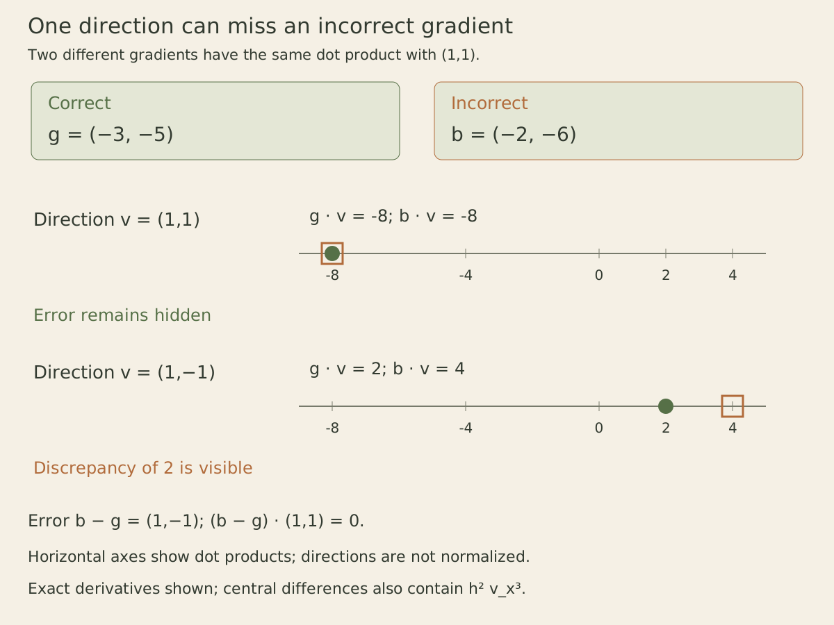

View full-size image ↗

Any error orthogonal to every direction tested is invisible to exact directional comparisons. Diverse directions and coordinate checks reduce that blind spot; they do not prove the implementation globally correct. Test representative inputs and separate parameter groups, including small bias vectors that uniform sampling might rarely select.

Even checking every coordinate at one input can miss a bug. Imagine a backward routine that adds x-1 to the correct x derivative. At our initial x value of one, the extra term vanishes. At (0,-2), the correct x derivative is −6 while that routine reports −7; a sufficiently small central step exposes the difference. Keep a second input that changes which terms are active, instead of treating one successful fixture as proof over the input domain.

For gradients spanning different magnitudes, a declared rule such as abs(a-n) <= atol + rtol * max(abs(a), abs(n)) combines absolute and relative tolerances. Check it per component, retain the actual values, and choose tolerances for the numeric scale. A huge correct component can hide a smaller wrong one in an aggregate norm. Passing both zero values is also uninformative if the input never changed.

Keep the same function, and recognize a kink

The CS231n gradient-checking notes emphasize centered differences, precision, representative inputs and control of dropout or augmentation. The useful principle is to compare the same function. Fix the data, random choices and mutable state for the positive evaluation, negative evaluation and derivative calculation. Resetting a seed alone does not restore running statistics or guarantee identical random consumption in a different branch.

For an explicit illustration, add 0.01 to the positive function call and −0.01 to the negative one. The resulting derivative error is 0.01/h in addition to truncation. At h=0.001, that artificial mismatch contributes ten. Equal additive offsets cancel in exact arithmetic; a fixed dropout mask is more complicated and must also be used by the derivative being checked.

ReLU introduces another boundary. At zero it has no ordinary derivative, yet a symmetric difference returns one half for every positive step. At −0.25 the derivative is zero, but a step of one crosses the kink and returns 0.375. A step of 0.125 stays entirely in the flat region and returns zero.

relu = lambda x: max(Q(0), x)
assert central(relu, (Q(0),), (1,), Q(1, 10)) == Q(1, 2)
assert central(relu, (Q(-1, 4),), (1,), Q(1)) == Q(3, 8)
assert central(relu, (Q(-1, 4),), (1,), Q(1, 8)) == 0
h = Q(1, 1000)
unequal_offsets = (Q(1, 100) - Q(-1, 100)) / (2*h)
assert unequal_offsets == 10
print('ReLU:', Q(1, 2), Q(3, 8), 0)
print('Extra error from unequal offsets:', unequal_offsets)

A library’s chosen backward value at the kink need not match that symmetric quotient. Check smooth regions and test the documented boundary convention separately. PyTorch explicitly warns about nondifferentiable inputs and overlapping tensor storage; aliased coordinates are not independent perturbations. Our scalar fixtures have neither shared storage nor stateful layers.

For an exercise, use direction (2,1). Derive its exact truncation term 8h², correct directional derivative −11 and buggy derivative −10, then rerun the comparison. Next replace the cubic coefficient with two and derive the coordinate error 2h² before changing the assertion. Finally, test the intended loss reduction independently: a correctly differentiated sum can pass every gradient check even when the application requires a mean. Agreement between a forward function and its derivative does not establish that the forward function expresses the right problem.