Likelihood is a function of the parameter
Derive a Bernoulli likelihood, compare sample-size effects and serial dependence, and reproduce why equal success counts need not mean equal sequence probabilities.
A likelihood treats the observations as fixed and asks how well different parameter values account for them. A probability model treats the parameter as specified and describes possible observations. The numerical formula can be the same, but the argument that is allowed to vary changes its meaning.
For a developer fitting a classifier, this distinction explains why maximizing likelihood is a training rule and why a likelihood curve is not automatically a probability distribution over model weights. A ten-trial Bernoulli example makes the distinction visible without a large dataset.
Keep the data fixed
Suppose ten independent binary trials produce seven successes and three failures. Assume every trial has the same unknown success probability p. If the exact observed sequence is the data, its probability under a specified p is:
P(observed sequence | p) = p^7 × (1 - p)^3For p = 0.5, this is 0.5^10, approximately 0.0009766. For p = 0.7, it is approximately 0.0022236. For p = 0.9, it is approximately 0.0004783. The observed sequence is more probable under 0.7 than under either alternative.
When those observations stay fixed and p varies, call the expression L(p), the likelihood. Every point on the curve evaluates the same data under a different candidate parameter. The curve’s height does not mean there is a 0.22% probability that p equals 0.7.
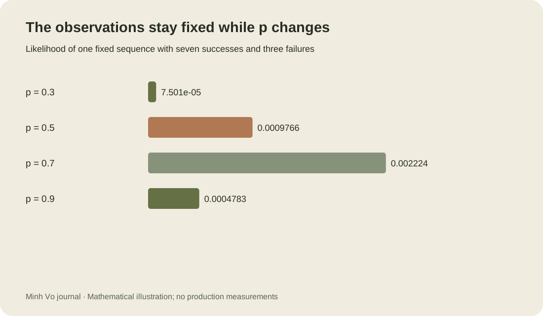
A small likelihood is normal when data include a specific sequence. There are many possible sequences, and each can have small probability. What matters for maximum-likelihood fitting is how the likelihood changes across parameter values for the same observations.
For the same fixed sequence, the candidate likelihoods can be compared directly:
| Candidate success probability | Sequence likelihood | Compared with p = 0.5 |
|---|---|---|
| 0.5 | 0.0009765625 | 1.000 |
| 0.7 | 0.0022235661 | 2.277 |
| 0.9 | 0.0004782969 | 0.490 |
A count changes a constant, not the maximizer
If the observation is only the total number of successes, the binomial probability includes the number of sequences with that count:
P(K = 7 | p) = choose(10, 7) × p^7 × (1 - p)^3
            = 120 × p^7 × (1 - p)^3
The constant 120 multiplies the likelihood at every candidate p. It changes the numerical probability of the observed event but leaves the maximizing parameter unchanged. It also leaves likelihood ratios between parameter values unchanged.
The distinction between a sequence and a count matters when reporting an actual probability. It often disappears from an optimization implementation because parameter-independent constants can be omitted. A training loss that omits constants can still choose the same model, while no longer being numerically equal to the full negative log probability of the stated observation.
Find the maximum with a derivative
Products of many probabilities can underflow in floating-point arithmetic. Taking logarithms turns products into sums and preserves their ordering because the logarithm is increasing. Omitting the binomial constant, the log likelihood is:
ell(p) = 7 log(p) + 3 log(1 - p)
ell'(p) = 7 / p - 3 / (1 - p)
Setting the derivative to zero gives 7(1 - p) = 3p, so p = 0.7. The second derivative is -7 / p² - 3 / (1 - p)², which is negative inside (0, 1). This stationary point is therefore the unique maximum in that interval. The general result is the observed success fraction k / n.
For all-success or all-failure samples, the maximum occurs at a boundary. That can produce probabilities exactly 1 or 0, which create infinite log loss if the next observation contradicts the estimate. A prior or a regularization rule can soften the boundary, but it changes the estimation procedure and should be described.
A likelihood ratio also has a useful scale interpretation. Here L(0.7) / L(0.5) is about 2.277. The observed sequence is about 2.277 times as probable under the first candidate as under the second. That is evidence comparing those two specified candidates; it does not supply their prior odds or account for candidates selected after inspecting the data.
The same estimate can come with different likelihood shapes
Compare the original seven successes in ten trials with a second hypothetical sample containing seventy successes in one hundred trials. Both have a maximum-likelihood estimate of 0.7. They do not supply the same evidence for every alternative parameter.
To compare shapes on one figure, divide each likelihood by its own maximum. The resulting relative likelihood has height one at 0.7 in both cases. For the ten-trial sample, the relative likelihood at 0.5 is about 0.4392. For the hundred-trial sample, it is that number raised to the tenth power, about 0.000267. The second sample more sharply distinguishes 0.5 from 0.7 under the same independent, constant-probability model.
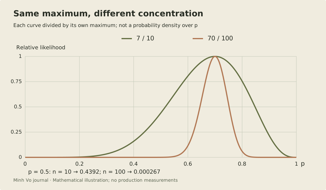
Scaling a curve to height one does not turn it into a probability density. Its area has not been normalized, and the horizontal coordinate still denotes a candidate parameter. The plotted curves describe relative fit to two different datasets. Do not compare their unscaled likelihood heights as a score for which dataset is better: multiplying more probabilities generally makes a sequence probability smaller.
The comparison also assumes the extra observations are informative new trials. Copying each of the original ten rows ten times yields the same algebraic product if a program blindly treats all rows as independent. It does not yield a hundred independent observations. The sharply concentrated curve would then reflect a false sampling model, much like an uncertainty estimate that treats duplicated records as new evidence.
This is why an unchanged point estimate does not settle whether an evaluation has improved. Examine the sampling process and the whole likelihood shape, while using a separate inferential method if you need a confidence interval or a posterior probability. The relative-likelihood plot alone supplies neither of those objects.
Discarding order depends on the model
The count-based shortcut worked because the assumed trials were independent with one shared success probability. Every ordering with seven successes then has the same probability. A model with serial dependence can distinguish those orderings, so a success count may discard information needed to evaluate it.
Consider two fixed sequences, SSSSSSSFFF and SFSFSFSSSS. Each contains seven successes and three failures. Under the original Bernoulli model at 0.7, both have probability approximately 0.0022236.
Now define a separate toy sequence model. The first symbol is equally likely to be S or F. Each later symbol repeats the previous one with probability 0.9 and switches with probability 0.1. These rules specify conditional probabilities for the next symbol; they are not an estimated model of a real event stream.
The first sequence has eight repeated-symbol transitions and one switch. Its probability is 0.5 × 0.9^8 × 0.1, about 0.0215234. The second sequence has three repeats and six switches. Its probability is 0.5 × 0.9^3 × 0.1^6, or 0.0000003645. Equal success counts no longer imply equal sequence probabilities.
The probability chain rule still works: multiply the first-symbol probability by the conditional probability of each next symbol given the relevant history. What failed was the independent-trial simplification. For a stream of repeated events, retain ordering and grouping information until the model’s assumptions justify discarding them. A parser that reduces every session to one success count can make some dependence models impossible to fit later.
Marco Taboga’s maximum-likelihood lesson defines likelihood using the joint distribution of the observed sample. That definition covers both examples. The product of identical Bernoulli terms is one particular joint model, not the definition of likelihood itself.
Reproduce the comparison without a model-training library
Write a short calculation that counts successes and failures in each fixed sequence. Evaluate the Bernoulli product at 0.5, 0.7 and 0.9, then compare the two sequences. Their likelihoods should match at every candidate because their counts match. Next count adjacent equal and unequal symbols and evaluate the conditional model above. The two sequence probabilities should now differ.
For the sample-size plot, calculate the log likelihood relative to its maximum and exponentiate the difference. This avoids dividing two very small products. Check that each curve reaches one at 0.7 and that the hundred-trial relative value at 0.5 equals the ten-trial value raised to the tenth power. Reject candidate probabilities outside zero to one, and handle boundary observations without evaluating a zero count times the logarithm of zero.
The exercise checks which data the computation uses, which observations it assumes independent, and which constants can be dropped. It does not prove that the Bernoulli or serial model fits an application. That requires evidence about the data-generating process and evaluation of predictions on appropriately held-out sequences.
A probability over parameters needs another ingredient
Bayesian inference combines likelihood with a prior distribution over the parameter. The posterior is proportional to L(p) × prior(p), then normalized over parameter values. The prior and the chosen parameterization are part of that construction. Merely drawing a likelihood curve does not supply them.
There is a subtle exception worth understanding: on a bounded one-dimensional parameter space, a particular likelihood can be normalized as a density with respect to a chosen measure. That corresponds to a particular prior choice, such as a uniform density in that coordinate. A uniform density in p is not uniform in its log odds, so “normalize the likelihood” is not a coordinate-free substitute for specifying the prior.
Deep Learning’s probability chapter provides the probability rules behind the model, and its machine-learning chapter develops maximum-likelihood estimation. When reading a model’s loss function, identify the observations, the parameter and any omitted constants. Those three details explain what the optimizer is actually maximizing.