Gradient descent on a quadratic you can solve exactly

Gradient descent on a positive quadratic is simple enough to solve exactly. That makes it a useful test of three claims that are easy to confuse: the parameters get closer to a minimum, the objective decreases, and a learning rate is stable from every starting point. Those claims can give different answers even on a two-variable problem.

If you are learning optimization, this lesson assumes you know derivatives and geometric sequences. We begin with one variable, then add a second curvature direction. All objectives and starting points are invented teaching cases. The calculations use exact rational arithmetic, so a numerical rounding artifact cannot explain an apparent success or failure.

The multiplier tells the whole one-variable story

Let the objective be f(x) = lambda*x²/2, where curvature lambda is positive. The minimum is zero, and the derivative is lambda times x. With a constant learning rate eta, gradient descent satisfies:

x_(t+1) = x_t - eta*lambda*x_t = (1-eta*lambda)*x_t
x_t = (1-eta*lambda)^t*x_0
f(x_t) = (1-eta*lambda)^(2t)*f(x_0)

For a nonzero starting point, convergence to the minimum requires the multiplier’s absolute value to be less than one. Solving that inequality gives the strict interval 0 < eta < 2/lambda. A smaller multiplier magnitude means faster contraction per step in this exact model.

At eta zero, nothing moves. At eta equal to twice the reciprocal curvature, the parameter changes sign without shrinking. Above that boundary, or at a negative rate, a nonzero starting point grows in magnitude. Starting exactly at zero is a special case: every rate leaves it there because the gradient is zero. A successful run from the optimum says nothing about the stability of nearby starts.

The Deep Learning optimization chapter distinguishes the optimization problem from the broader learning problem. Our derivation concerns the objective being optimized. Reaching its minimum does not establish generalization to unseen data.

A falling objective can hide alternating parameters

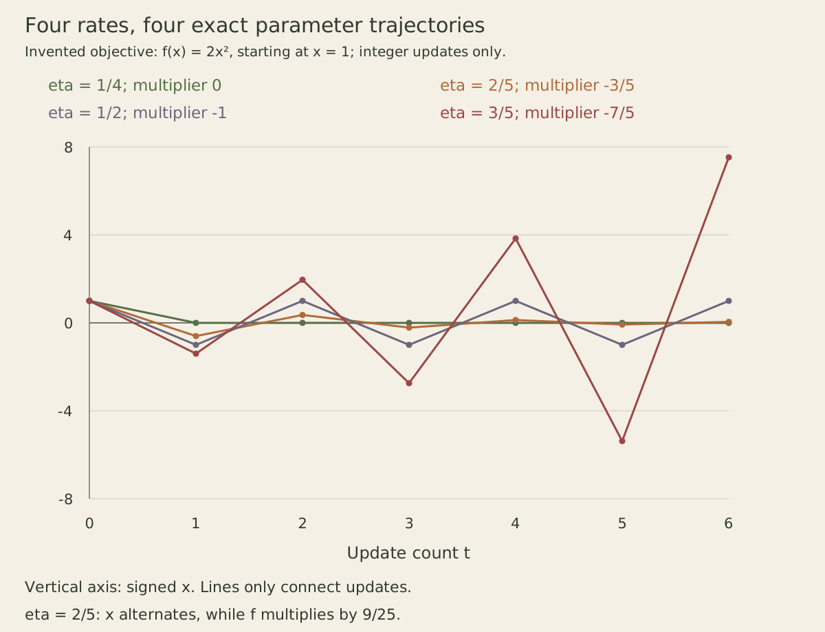
Use f(x)=2x², so curvature is four, and start at one. The stable interval is zero to one half, excluding both endpoints. Four rates expose different behavior:

Rate	Multiplier	First three values after the start	Behavior
1/4	0	0, 0, 0	Reaches zero in one update
2/5	−3/5	−0.6, 0.36, −0.216	Alternates and converges
1/2	−1	−1, 1, −1	Alternates at fixed magnitude
3/5	−7/5	−1.4, 1.96, −2.744	Alternates and diverges

Run the three Python blocks in order in one session. They need only the standard library. Keep the learning rate and curvature separate in the interface: their product controls the recurrence.

from fractions import Fraction as F

def trajectory(curvature, rate, start, steps):
    x = F(start)
    values = [x]
    for _ in range(steps):
        x = x-rate*curvature*x
        values.append(x)
    return values

rates = [F(1,4), F(2,5), F(1,2), F(3,5)]
for rate in rates:
    values = trajectory(F(4), rate, F(1), 6)
    print(rate, values[:4])
    multiplier = 1-4*rate
    assert values == [multiplier**t for t in range(7)]

At rate 2/5, the signed parameter multiplier is minus 3/5 but the objective multiplier is 9/25. Every objective value falls to 36% of the preceding one while the parameter crosses the optimum each time. Oscillation alone is not divergence; losing the sign in the objective plot can conceal perfectly stable oscillation.

The written adaptation of Grant Sanderson’s October 16, 2017 lesson, by Josh Pullen, introduces the negative gradient through the direction of steepest descent. Direction is local information; the learning rate determines how far a finite update travels. The exact multiplier here checks that additional choice.

The one-step solution at rate 1/4 is also special. It uses the exact curvature of this quadratic. A nonlinear objective can have different curvature at the next position, so estimating a convenient rate at one point does not establish the same recurrence throughout training.

View full-size image ↗

One rate must serve every active direction

Now use g(x,y)=(x²+9y²)/2. The gradient is (x,9y). A simultaneous update scales x by 1-eta and y by 1-9eta. To converge from every starting point, both magnitudes must be below one, which requires 0 < eta < 2/9.

The qualifier “every” matters. A coordinate initially equal to zero remains zero in this exact diagonal system. A rate can therefore succeed from a specially aligned start while being unstable in a direction that the run never explores.

def plane(rate, start, steps):
    x, y = map(F, start)
    states = [(x,y)]
    for _ in range(steps):
        x, y = x-rate*x, y-9*rate*y
        states.append((x,y))
    return states

def objective(state):
    x, y = state
    return (x*x+9*y*y)/2

aligned = plane(F(1), (1,0), 5)
perturbed = plane(F(1), (1,F(1,1000)), 5)
print('aligned after one update:', aligned[1])
print('perturbed steep coordinate:', [y for x,y in perturbed])
assert aligned[1] == (0,0)
assert abs(perturbed[-1][1]) == F(4096,125)

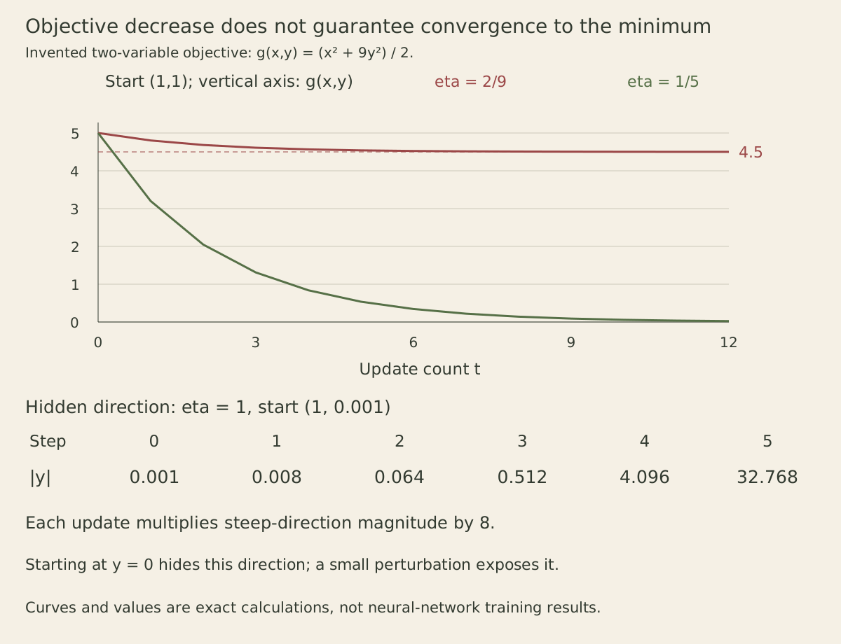
Rate one takes the aligned start (1,0) directly to the minimum. Adding just 0.001 in the steep direction changes the story: that coordinate is multiplied by minus eight at every update. After five updates its magnitude is 32.768. The original successful trajectory did not certify a neighborhood of stable behavior.

For a general symmetric positive-definite quadratic, an orthonormal eigenvector basis gives the same calculation, with one multiplier for each Hessian eigenvalue. Stability from every start uses the largest eigenvalue. For a particular exact starting error, only directions with a nonzero component participate. Noise, finite precision or a change to the objective can introduce components absent from an idealized calculation.

Deep Learning’s numerical-computation chapter explains conditioning and curvature in gradient-based optimization. The two-direction example makes that geometry explicit without treating an observed gradient magnitude as a curvature estimate.

Strictly decreasing values can still stop above the minimum

Set the rate to the boundary 2/9 and start at (1,1). The shallow coordinate contracts by 7/9, but the steep coordinate alternates between one and minus one. The objective after t updates is 9/2 + (7/9)^(2t)/2.

This sequence is strictly decreasing at every finite step, yet its limit is 4.5 while the minimum is zero. Small changes in the objective eventually reflect the dying shallow component, not successful optimization of the steep component. A stopping rule based only on the change in loss can mistake stagnation above the optimum for convergence.

By contrast, rate 1/5 gives coordinate multipliers 4/5 and minus 4/5. From (1,1), the objective equals 5*(16/25)^t and tends to zero. It still oscillates in the steep coordinate, but both components shrink.

boundary = plane(F(2,9), (1,1), 12)
stable = plane(F(1,5), (1,1), 12)
for t in range(13):
    assert objective(boundary[t]) == F(9,2)+F(1,2)*F(7,9)**(2*t)
    assert objective(stable[t]) == 5*F(16,25)**t
print('boundary after twelve:', float(objective(boundary[-1])))
print('stable after twelve:', float(objective(stable[-1])))
assert all(objective(boundary[t+1]) < objective(boundary[t]) for t in range(12))

The gradient norm provides a different diagnostic here: its steep component keeps magnitude nine on the boundary trajectory. That diagnostic also needs scale awareness. A small gradient can arise from a small objective normalization, and a large constant added to the objective changes its displayed value without changing any gradient. Compare quantities whose meaning is specified, not only convenient plotting scales.

View full-size image ↗

The fastest robust rate is a different question from a lucky first step

For the two curvatures one and nine, the worst coordinate contraction factor is the larger of |1-eta| and |1-9eta|. The smallest possible worst factor is 4/5, achieved at eta 1/5. If both magnitudes were strictly below 4/5, the shallow direction would require eta above 1/5 while the steep direction would require eta below 1/5, a contradiction.

This minimizes the worst contraction over starting directions for a constant rate. It does not promise the smallest objective after every fixed number of updates from every start. From (1,0), rate one wins immediately, but lacks stability in nearby steep directions. A claim about “the best learning rate” needs to specify which of these objectives it means.

Rescaling changes the numerical rate

Multiplying the entire objective by a positive constant c multiplies its gradient and curvature by c. Dividing the learning rate by c preserves each update exactly. This is why switching a summed loss to its mean changes the effective step unless the learning rate is adjusted consistently.

A coordinate change is different. If x=s*u with nonzero s, the same scalar objective written in u has curvature lambda*s². A step of size alpha in u becomes a step of size alpha*s² in x after conversion back. Matching the original x trajectory therefore requires alpha equal to eta divided by s squared. Merely renaming units while retaining the numeric learning rate changes the algorithm.

For an exercise, multiply the scalar objective by ten and verify identical trajectories after dividing every rate by ten. Then use x=2u, start at u=1/2, and check that rate 1/10 in u reproduces the x trajectory at rate 2/5. Finally use the two-variable boundary rate with start (1,0) and then (1,1). The first converges; the second does not. Record the initial direction, objective normalization and convergence criterion before using a curve as evidence that an optimizer is stable.