Read residuals before adding another model

A residual is the observed target minus the fitted prediction. Plotting residuals against inputs or fitted values can reveal patterns that an aggregate score hides. Curvature suggests that the fitted mean function is missing structure; a changing vertical spread suggests that uncertainty varies with the input.

If you have fitted a regression and want to understand its mistakes, start with the residuals in their original units.

Residual patterns have a limitation: several different causes can produce similar shapes. Data errors, omitted variables, dependence and a poorly chosen evaluation split can produce patterns too. Start by tracing what the plotted points actually represent.

Fit a line to a curved target

Use five hypothetical observations with x = -2, -1, 0, 1, 2 and y = 4, 1, 0, 1, 4. The target is exactly x². Fit ordinary least squares with an intercept and a linear x term.

The mean of x is zero, and the mean of y is 2. The slope is the centered cross-product divided by the centered input sum of squares. Symmetry makes the numerator zero:

sum x_i (y_i - 2) = (-2)(2) + (-1)(-1) + 0(-2) + 1(-1) + 2(2)
                  = 0
slope = 0 / 10 = 0
intercept = 2

The fitted line predicts 2 everywhere. Residuals are 2, -1, -2, -1, 2. Their sum is zero, as ordinary least squares with an intercept requires on its training sample. That zero sum does not mean the residuals lack structure.

View full-size image ↗

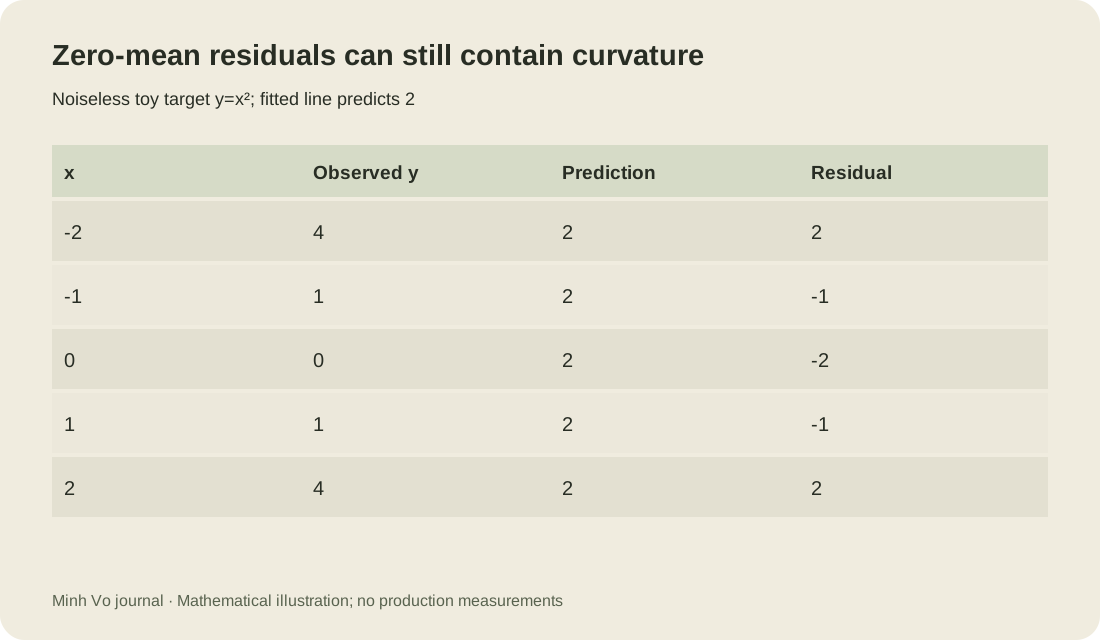
Both ends sit above the fitted line, while the center sits below it. Adding the feature x² lets a linear-in-parameters regression represent the target exactly in this noiseless toy dataset. The model is linear in its coefficients even though the feature is a nonlinear function of the original input.

Separate model structure from noise structure

The example’s curvature concerns the conditional mean. A second kind of pattern concerns residual spread. Imagine repeated measurements at each input where noise standard deviation is 1 near zero and 4 at the edges, while the mean function is correctly specified. Residuals can average near zero at every input but fan outward toward the edges.

That hypothetical fan suggests heteroscedasticity, meaning conditional noise variance changes with the input. Adding a quadratic mean term does not necessarily fix it. You might need a model for conditional variance, a transformation justified by the target, or an uncertainty method that accounts for the changing spread.

Do not infer these properties from five single observations with confidence. The tiny example demonstrates geometry. With real data, repeated observations or enough local coverage are needed to distinguish noise from systematic structure. A smooth residual curve can also overfit when the dataset is small.

Training residuals are partly constrained by fitting

Least squares chooses coefficients using the training targets. Its residuals therefore have algebraic relationships with the fitted feature columns. With an intercept, their mean is zero up to numerical precision. With full-rank ordinary least squares, residuals are orthogonal to the columns of the design matrix.

Those relationships are not a guarantee of generalization. Plot held-out residuals too, preferably with predictions generated under a split that matches deployment. Cross-fitted predictions can give a broader diagnostic view while keeping each observation out of the fit that predicts it.

Scikit-learn’s linear-model guide describes ordinary least squares and notes its sensitivity to correlated design columns. A residual plot complements that model definition by exposing what the fitted predictions leave unexplained.

Check the axes before interpreting a pattern

A residual-versus-time plot can reveal drift or a delayed feature problem. A residual-versus-prediction plot can reveal mean or variance patterns across the model’s output range. A residual-versus-feature plot can reveal a missing interaction. Each plot answers a different question, so keep the axis labels and units explicit.

High-leverage inputs deserve attention because they can strongly influence the fit. A point far from the rest of the input cloud may pull the line toward itself and end up with a modest residual. Residual size alone does not measure influence. Investigate the input position, measurement provenance and effect of leaving the point out before deciding it is an outlier to remove.

A point can pull its own fitted residual toward zero

Consider four constructed observations: (0,0), (1,1), (2,2) and (10,20). The first three lie exactly on y=x. The last input is far from the others, so it can strongly affect the fitted slope. Compute both the fit using all four observations and the fit using only the first three.

from fractions import Fraction as F

def fit_line(xs, ys):
    xbar = sum(xs) / len(xs)
    ybar = sum(ys) / len(ys)
    spread = sum((x-xbar)**2 for x in xs)
    slope = sum((x-xbar)*(y-ybar) for x, y in zip(xs, ys)) / spread
    return ybar-slope*xbar, slope

xs = list(map(F, [0, 1, 2, 10]))
ys = list(map(F, [0, 1, 2, 20]))
a, b = fit_line(xs, ys)
predictions = [a+b*x for x in xs]
residuals = [y-p for y, p in zip(ys, predictions)]
print('full coefficients:', str(a), str(b))
print('full residuals:', [str(e) for e in residuals])
a_other, b_other = fit_line(xs[:-1], ys[:-1])
print('other-three prediction at 10:', str(a_other+b_other*xs[-1]))
print('left-out error:', str(ys[-1]-a_other-b_other*xs[-1]))
assert sum(residuals) == 0
assert sum(x*e for x, e in zip(xs, residuals)) == 0

The full-fit intercept is -250/251 and its slope is 521/251, about 2.076. Its residuals are 250/251, -20/251, -290/251, 60/251. The last point has a residual of only about 0.239. The point at x=2 has a larger residual magnitude, about 1.155, even though the first three points lie on a perfectly straight line together.

When the last point is excluded, the other three give intercept zero and slope one. Their prediction at x=10 is 10, so the excluded observation’s prediction error is 10. The small residual from the full fit hid how much that observation helped determine its own fitted value. A residual threshold alone would focus on the wrong geometric question.

View full-size image ↗

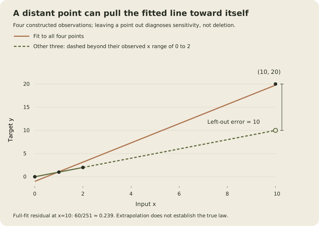
Excluding a point is a diagnostic here, not a recommendation to delete it. The observation might be valid and reveal that the relation changes at large inputs. It might instead have an incorrect label, unit or feature timestamp. Check its provenance and collect relevant examples before deciding. The other-three prediction at x=10 also extrapolates far beyond their observed range, zero through two. Its large error demonstrates sensitivity; it does not certify that y=x is the true law at ten.

Give leverage an operational meaning

For simple least squares with an intercept, the leverage of observation i is h_i = 1/n + (x_i-xbar)² / sum_j (x_j-xbar)². It depends on the observed inputs, not the labels. One interpretation follows directly from the fitting formula: if only label i changes by one unit while the inputs stay fixed, its own fitted value changes by h_i units.

In this example the leverage at x=10 is 245/251, about 0.976. Its own residual therefore changes by only 6/251 when its label changes by one. Much of the label change is absorbed into the fitted prediction. This is why a distant point can have a small training residual and substantial influence on the fit at the same time.

The statsmodels OLS influence reference distinguishes hat-matrix diagonals, residual measures and fits that leave one observation out. These measure related but different properties. The calculation above uses exact scalar arithmetic; it does not claim to run that library or turn a diagnostic threshold into a data-deletion rule.

The helper assumes finite equal-length inputs, at least two observations and positive input spread. If all inputs are equal, a separate intercept and slope are not uniquely determined. Removing a point can also leave a degenerate design. Recognize that loss of identifiability instead of reporting a division-by-zero failure as evidence that the omitted point was erroneous.

Exercises that distinguish fit constraints from predictive evidence

Change only the last target from 20 to 21 and refit. Verify that its fitted value rises by 245/251, while its residual rises by 6/251. Then fit all four leave-one-out models. Each point’s diagnostic prediction must come from the other three, rather than from a model that already used that point’s label. For these four distinct inputs, every reduced design still has positive spread.

Return to the first quadratic example and add 5 to every target. The fitted intercept increases from 2 to 7, the slope stays zero and the training residuals stay exactly the same. A residual plot can therefore hide an overall target-level change when the model is refitted to it. If the original line at 2 is instead frozen and used on those shifted targets, the prediction errors each increase by 5. Name whether the displayed fit was retrained before attributing a residual change, or its absence, to stability.

Finally, create repeated observations at each of x=-1,0,1 with targets x-2 and x+2. The fitted mean relation is y=x; the residual spread is the same at every input. Replace the two edge pairs by x-4 and x+4, leaving the center pair unchanged. The mean relation still fits, but edge residual magnitudes double. This stipulated construction separates a spread change from missing curvature without pretending that six observed values would establish a noise law in a real application.

Turn the pattern into a testable revision

For the quadratic toy example, the proposed revision is concrete: add x², fit using training data and compare held-out squared error under the same split. For a suspected missing interaction, specify the interacting variables and the observation that motivates them. Avoid searching many transformations against the final test set.

Retain the simple model as a comparator. A more flexible fit may reduce visible training curvature while becoming unstable outside the observed range. Predictions far beyond x = -2 to 2 are unsupported by this five-point exercise. A diagnostic has done its job when it leads to a specific hypothesis and an evaluation that could reject that hypothesis.