Backpropagation adds every path through a computation
Trace a shared scalar computation, reproduce its gradients, expose a detached branch and distinguish a ReLU kink from a gradient bug.
One intermediate value can influence a loss through several paths. Backpropagation must add those contributions before sending the result farther upstream. In the small network below, keeping only the hidden-layer path gives a weight derivative of 24. Keeping the direct path as well gives the correct derivative of 32, even though both programs report the same forward loss of 8.
This article is for students and engineers learning how automatic differentiation works. You should know the derivative of a product and be able to run small Python functions. We will build a scalar reference, inspect its actual values and gradients, and test a ReLU boundary. The inputs are invented for this lesson; no training dataset, accelerator measurement or framework execution is involved.
Give every intermediate a meaning
Fix the input at x = 2, the target at 1, and parameters w = 1, b = −1, v = 3. Compute p = w*x, z = p+b, h = max(0,z), q = v*h, and y = q+p. The direct addition of p reuses the same intermediate that feeds the hidden unit. It is a deliberately small shared computation, not an assertion about a particular residual-network architecture.
Use the half-squared loss L = (y−target)^2/2. The forward values are p=2, z=1, h=1, q=3 and y=5. The error is 4 and the loss is 8. At this point the ReLU is strictly active, so its ordinary derivative is 1. These saved values determine the local derivatives needed on the reverse pass.
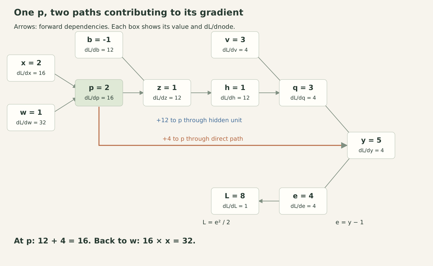
Arrows describe the actual toy computation. The reverse contributions reaching p are 12 through the hidden unit and 4 through the direct addition.
Start from dL/dL = 1. The loss sends error 4 back to y. Addition sends that same 4 to q and directly to p. Multiplication by v sends 4*v = 12 to h, and the active ReLU passes 12 to z. The addition forming z sends 12 more to p and 12 to b. Therefore dL/dp = 4+12 = 16. Multiplication forming p gives dL/dw = 16*x = 32 and dL/dx = 16*w = 16. The output weight receives dL/dv = 4*h = 4.
This is the multivariable chain rule at a shared node: sum the contribution from every downstream use. A node’s own derivative with respect to its parent is a local quantity; its accumulated gradient measures the effect on the chosen final loss. Confusing those two numbers is an easy way to miss a factor or a branch.
Dive into Deep Learning’s forward/backward chapter develops this reverse dependency order and reuse of forward intermediates. Its example also shows separate contributions from a data loss and a regularizer. Our scalar example uses a direct output path instead, so every contribution can be checked numerically.
Implement local rules and accumulate their contributions
The following four Python blocks run in order in one session. This small reference supports addition, multiplication and ReLU. A pullback distributes an output’s accumulated gradient to the inputs of one operation. The additions inside these functions are essential.
class Value:
    def __init__(self, value, parents=()):
        self.value = float(value)
        self.grad = 0.0
        self.parents = parents
        self.pullback = lambda: None

    @staticmethod
    def wrap(value):
        return value if isinstance(value, Value) else Value(value)

    def __add__(self, other):
        other = self.wrap(other)
        out = Value(self.value + other.value, (self, other))
        def pullback():
            self.grad += out.grad
            other.grad += out.grad
        out.pullback = pullback
        return out

    def __mul__(self, other):
        other = self.wrap(other)
        left, right = self.value, other.value
        out = Value(left * right, (self, other))
        def pullback():
            self.grad += right * out.grad
            other.grad += left * out.grad
        out.pullback = pullback
        return out

    def relu(self):
        active = self.value > 0
        out = Value(max(0.0, self.value), (self,))
        def pullback():
            self.grad += out.grad if active else 0.0
        out.pullback = pullback
        return out

    def backward(self):
        order, visited = [], set()
        def visit(node):
            if node in visited:
                return
            visited.add(node)
            for parent in node.parents:
                visit(parent)
            order.append(node)
        visit(self)
        for node in order:
            node.grad = 0.0
        self.grad = 1.0
        for node in reversed(order):
            node.pullback()

    __radd__ = __add__
    __rmul__ = __mul__
The traversal visits each node once, while each operation still distributes a contribution for every operand position. If the same node appears twice in a multiplication, it must receive both terms. Deduplicating the traversal is safe; discarding a repeated operand’s derivative is not. For r*r at r=3, those terms are 3 and 3.
Karpathy’s micrograd engine provides a compact educational implementation of this pattern, including addition into gradient fields and reverse topological traversal. This reference follows those ideas but explicitly clears every reachable gradient at the start of each backward call. It also captures multiplication values and the ReLU branch during the forward computation. These choices define this example’s behavior; they do not describe every automatic-differentiation API.
We build a fresh graph whenever parameters change. Do not edit node values or parent links inside a completed graph and expect its stored forward calculation to become a new evaluation. The class is intentionally small: it has no tensors, broadcasting, higher derivatives, checkpointing or general nonfinite-input policy. Its recursive traversal is suitable for this short graph, not an unbounded chain.
def network(w=1.0, b=-1.0, v=3.0, x=2.0, target=1.0, detach_skip=False):
    x, w, b, v = [Value(t) for t in (x, w, b, v)]
    p = w * x
    z = p + b
    h = z.relu()
    q = v * h
    skip = Value(p.value) if detach_skip else p
    y = q + skip
    e = y + (-target)
    loss = 0.5 * e * e
    return dict(x=x, w=w, b=b, v=v, p=p, z=z, h=h, q=q, y=y, e=e, loss=loss)

full = network()
full['loss'].backward()
print('forward', {k: full[k].value for k in ('p', 'z', 'h', 'q', 'y', 'e', 'loss')})
print('gradients', {k: full[k].grad for k in ('p', 'w', 'b', 'v', 'x')})
assert [full[k].grad for k in ('p', 'w', 'b', 'v', 'x')] == [16, 32, 12, 4, 16]
full['loss'].backward()
assert full['w'].grad == 32
broken = network(detach_skip=True)
broken['loss'].backward()
print('detached skip', 'loss', broken['loss'].value, 'w gradient', broken['w'].grad)
assert broken['loss'].value == 8 and broken['w'].grad == 24
r = Value(3)
(r * r).backward()
print('repeated operand', 'value', r.value, 'gradient', r.grad)
assert r.grad == 6
The complete run prints gradients p=16, w=32, b=12, v=4 and x=16. Calling this reference’s backward again returns the same values because it resets its buffers. Deliberate accumulation across examples would require a separate policy, including whether the objective sums or averages those examples.
The detached run wraps p’s current numeric value in a new leaf before the direct addition. Forward arithmetic still produces loss 8, but that new leaf has no recorded dependency on w. The remaining hidden path produces a weight gradient of 24. Automatic differentiation follows the graph it receives. Here, rebuilding the detached wrapper at each perturbed w also recomputes the copied p value, so the wrapper’s ordinary finite difference is still 32. The reported 24 is the derivative of the recorded graph with that copied leaf held constant; it is not the ordinary derivative of the wrapper that rebuilds the copy.
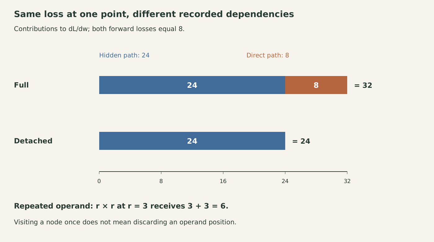
The hidden path contributes 24 to the weight derivative and the direct path contributes 8. Replacing the direct path by its numeric value removes its recorded derivative contribution.
A single forward evaluation and one reverse traversal compute all the scalar input gradients here. Their operation count follows the graph’s nodes and edges. By comparison, a central finite-difference check ordinarily needs two fresh loss evaluations for each checked parameter. This explains the reuse benefit without promising a particular speedup: tensor kernels, memory traffic and execution overhead are outside this experiment.
Check smooth points and kinks differently
At the original parameters, changing w slightly keeps the ReLU active. The local loss is a quadratic function of w, so its symmetric finite difference has no truncation error in exact arithmetic while both evaluations remain in that branch. The executed floating-point values are close to 32, with small arithmetic rounding.
Now set b to −2 while keeping w=1. The preactivation is exactly zero. Immediately to the left, the hidden output stays zero and the weight derivative approaches 2. Immediately to the right, the hidden path becomes active and the derivative approaches 8. There is no single ordinary derivative at that point.
def loss_at(w, b=-1.0):
    return network(w=w, b=b)['loss'].value

smooth_checks = []
for step in (1e-2, 1e-4, 1e-6):
    central = (loss_at(1 + step) - loss_at(1 - step)) / (2 * step)
    smooth_checks.append((step, central))
    assert abs(central - 32) < 1e-6
print('smooth central differences', [(h, round(d, 9)) for h, d in smooth_checks])
kink = network(b=-2.0)
kink['loss'].backward()
print('kink chosen w gradient', kink['w'].grad)
kink_checks = []
for step in (1e-2, 1e-4, 1e-6):
    base = loss_at(1, b=-2)
    left = (base - loss_at(1 - step, b=-2)) / step
    right = (loss_at(1 + step, b=-2) - base) / step
    central = (loss_at(1 + step, b=-2) - loss_at(1 - step, b=-2)) / (2 * step)
    kink_checks.append((step, left, right, central))
print('kink differences', [tuple(round(t, 9) for t in row) for row in kink_checks])
assert kink['w'].grad == 2
assert abs(kink_checks[-1][1] - 2) < 1e-4
assert abs(kink_checks[-1][2] - 8) < 1e-4
assert abs(kink_checks[-1][3] - 5) < 1e-4
Our ReLU rule chooses zero for its own derivative at zero, so the direct path remains and the returned weight gradient is 2. The central finite difference tends to 5 because it spans both sides. Its disagreement with 2 is not evidence that the accumulation code is broken. A finite difference has to be interpreted against the function’s local differentiability.
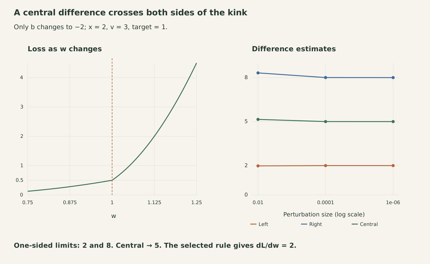
The kink experiment changes only b to −2. The left and right limiting derivatives are 2 and 8; the central difference approaches 5, while the declared reverse rule returns 2 at the boundary.
PyTorch’s autograd mechanics note explicitly distinguishes ordinary derivatives from conventions for nondifferentiable elementary operations. We use its discussion to frame this limitation, not as evidence of a PyTorch run. Our selected local ReLU rule is stated in the code, and no universal chain rule for arbitrary nonsmooth compositions is claimed.
For a practical gradient check, first choose a point away from known branch boundaries. Compare several perturbation sizes, inspect both absolute and relative error, and keep the loss definition and graph construction unchanged. Very small perturbations can lose information through subtraction and rounding. If the two sides activate different branches, inspect the one-sided behavior before treating a central estimate as a reference derivative.
A correct gradient does not select a safe step
The reverse pass gives derivatives, not a new parameter vector. The next block changes w, b and v simultaneously using the same original gradient. It holds x and the target fixed and recomputes the graph after the update. This separates differentiation from the optimizer decision.
updates = []
for rate in (0.01, 0.1):
    fresh = network()
    fresh['loss'].backward()
    parameters = {k: fresh[k].value - rate * fresh[k].grad for k in ('w', 'b', 'v')}
    after = network(**parameters)
    updates.append(dict(rate=rate, parameters=parameters, loss=after['loss'].value, hidden=after['h'].value))
print('one-step updates', updates)
assert updates[0]['loss'] < 8 < updates[1]['loss']
With rate 0.01, the new parameters are approximately w=0.68, b=−1.12 and v=2.96. The recomputed loss is about 0.57287808. With rate 0.1, they become −2.2, −2.2 and 2.6, and the loss rises to 14.58. The latter update crosses the activation boundary. The original gradient is still correct at the original point; it does not promise improvement for an arbitrary finite step.
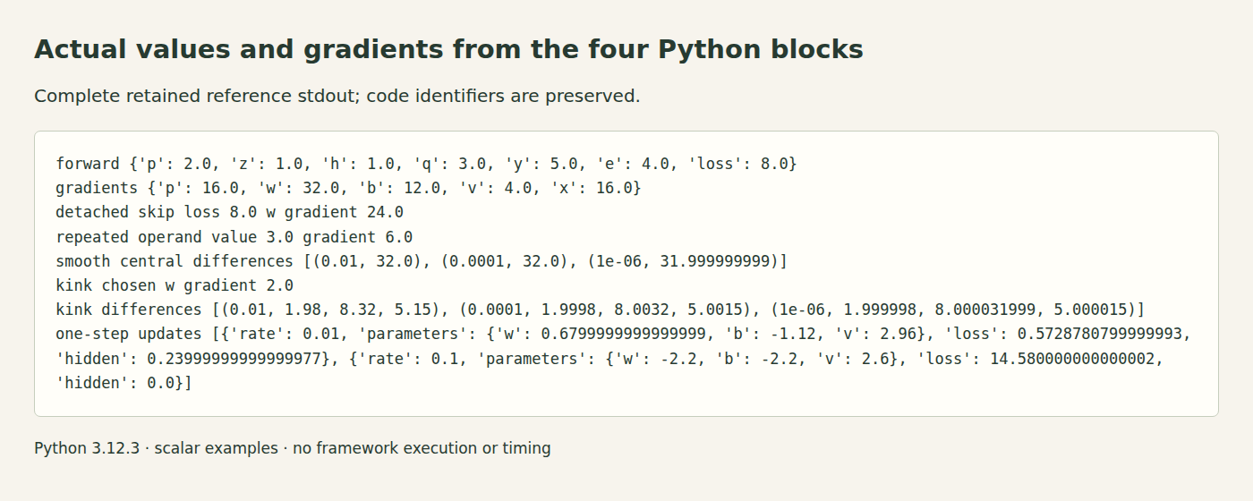
This local browser capture presents retained stdout from the four executed blocks. Labels identify the actual scalar experiment; it is not a training dashboard.
For an exercise, remove the direct output path entirely and use only y=q. At the original parameter values, expect loss 2 and derivatives w=12, b=6 and v=2. This changes both the forward function and its derivatives, unlike the detached experiment, which preserves one forward value while changing the recorded dependency.
Then restore the direct path and set v to zero. Expect loss 0.5, weight derivative 2, bias derivative 0 and output-weight derivative 1. A zero output weight blocks the hidden path’s current contribution to earlier parameters, but it does not prevent the output weight itself from receiving a gradient. Check those statements with a fresh graph and the stated target rather than carrying old buffers between exercises.