Expected loss and variance from a tiny discrete distribution
Calculate expected loss, variance and the distribution of a two-case average, then test how copied observations and rare large failures change the evaluation.
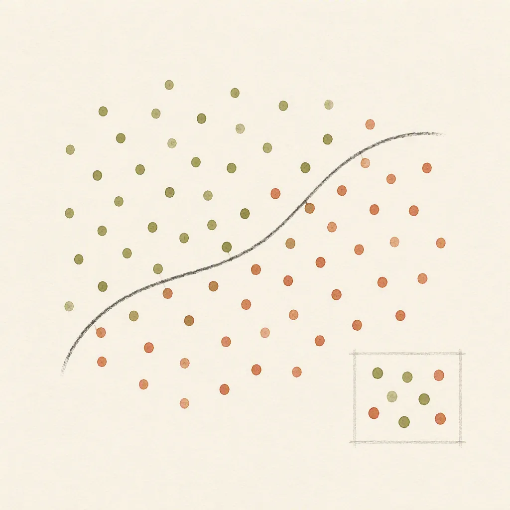
Expected loss averages a model’s errors across a specified distribution. Variance describes how much those errors fluctuate around that average. Two predictors can have equal expected loss and very different behavior on individual cases, so an average alone may be a poor description for a system with expensive large mistakes.
If you are choosing an evaluation metric, this distinction helps you decide which failures an average would conceal.
This article uses a discrete toy example. It needs only weighted sums, but the same distinction appears in evaluation dashboards, training objectives and decisions about a model’s worst failures. The losses below are abstract units, not probabilities and not an empirical benchmark.
Two predictors with the same average
Predictor A incurs loss 2 on every case. Predictor B incurs loss 0 with probability 0.9 and loss 20 with probability 0.1. The expected value of a discrete random variable is the sum of each possible value multiplied by its probability.
E[L_A] = 2 × 1 = 2
E[L_B] = 0 × 0.9 + 20 × 0.1 = 2
If the deployment objective really is to minimize expected loss, and these distributions are known exactly, the two predictors tie. Selecting B because it is perfect 90% of the time introduces a preference that the stated average-loss objective did not contain. Selecting A because its loss is predictable also introduces an additional preference. Both can be reasonable, but the evaluation rule should make that preference explicit.
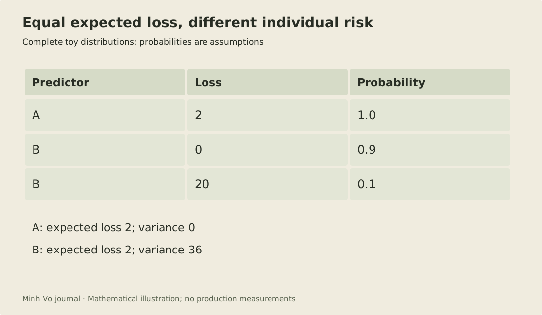
The table describes the complete hypothetical distributions. It does not claim that ten observed examples would contain exactly one high-loss event. Probabilities govern repeated sampling; a particular finite sample can look different.
Calculate spread in the same units
Variance is E[(L - E[L])²]. For A, every deviation from the mean is zero, so variance is zero. For B, the loss is either 2 below its mean or 18 above it.
Var(L_B) = 0.9 × (0 - 2)² + 0.1 × (20 - 2)²
         = 0.9 × 4 + 0.1 × 324
         = 36
SD(L_B)  = sqrt(36) = 6
Variance has squared loss units. Standard deviation returns to the original units. The equivalent identity Var(L) = E[L²] - E[L]² gives 40 - 4 = 36 for B and is convenient for checking the arithmetic. The probability chapter of Deep Learning states these definitions and distinguishes variance from other descriptions of a distribution.
Standard deviation does not tell you which side contains the large deviation. B’s distribution is asymmetric: many zeros and a few large positive losses. A histogram or a table preserves that information. Reporting the standard deviation beside the mean helps, but it does not reconstruct the tail.
Average loss also has sampling uncertainty
If you evaluate B on n independent cases from this same distribution, the variance of its sample mean is 36 / n. With 100 independent cases, the standard deviation of the sample mean is 0.6. With 10,000 cases it is 0.06. These quantities describe uncertainty in the estimated average, which differs from the spread of individual losses, still 6.
The independence assumption matters. Repeated frames from one video may share the same failure mode. Treating them as independent cases can make the average look more precisely estimated than it is. Decide whether the sampling unit is a frame, a video or a person before applying the 1 / n variance reduction.
There is also a substantial chance of seeing no high-loss case in a small sample. For ten independent cases under B, that probability is 0.9^10, about 34.9%. A ten-case demo can therefore report zero observed loss from a predictor whose true expected loss is 2. That does not invalidate small tests; it tells you what their evidence cannot establish.
Work out the distribution of a two-case average
The formula for an average is easier to understand after enumerating a small case. Draw two independent losses from predictor B and average them. There are four ordered outcomes: both are zero, only the first is twenty, only the second is twenty, or both are twenty. Independence lets you multiply the two marginal probabilities for each outcome.
| First loss | Second loss | Joint probability | Average loss |
|---|---|---|---|
| 0 | 0 | 0.81 | 0 |
| 0 | 20 | 0.09 | 10 |
| 20 | 0 | 0.09 | 10 |
| 20 | 20 | 0.01 | 20 |
Combining the two middle rows gives probabilities 0.81, 0.18 and 0.01 for average losses zero, ten and twenty. The expected average is still two. Its second moment is 0.18 × 100 + 0.01 × 400 = 22; subtracting the squared mean gives variance 18. Averaging two independent observations halves the original variance of 36.
Now draw one loss and copy it into both rows. Each row separately still has B’s distribution, but the pair is perfectly dependent. The average is zero with probability 0.9 and twenty with probability 0.1, exactly like one observation. Its variance remains 36. The row count doubled without adding independent information.
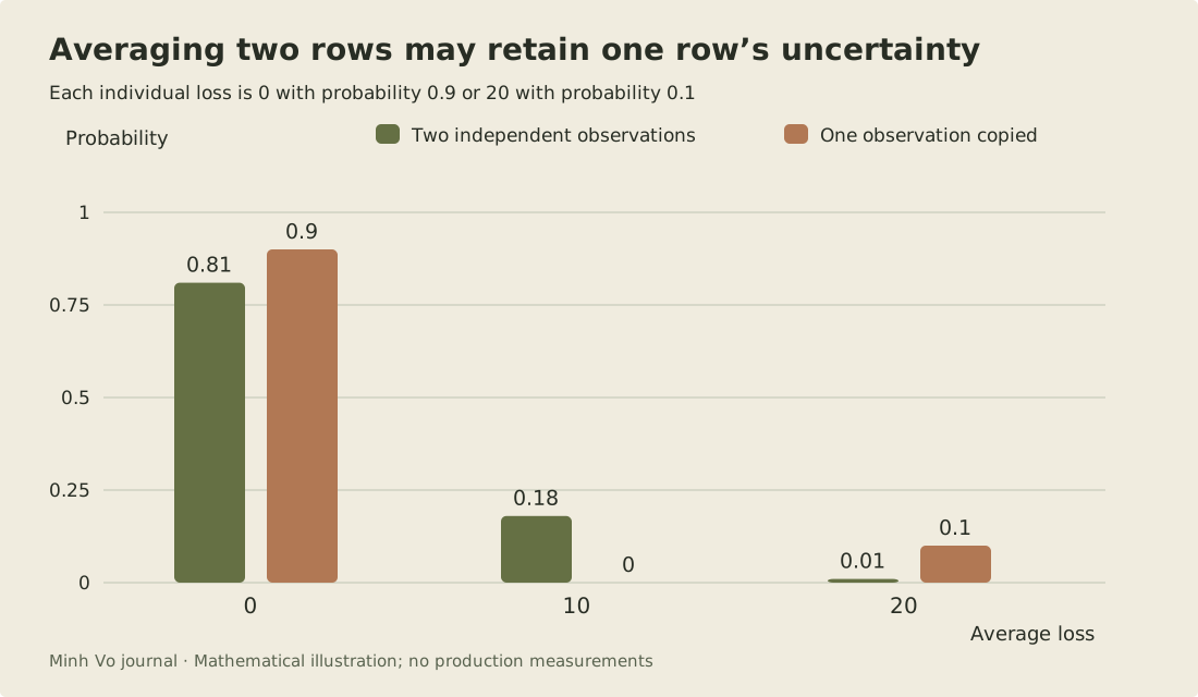
The second figure compares distributions of an average, not distributions of an individual prediction. It exposes why duplicating records or measuring two nearly identical frames does not automatically improve precision. Independence is a property of how observations arise, not a property created by putting them in separate table rows.
The general two-variable formula includes covariance: the variance of their average equals one quarter of the sum of their two variances plus twice their covariance. Here that is 18 + 0.5 Cov(L1,L2). Independent losses have zero covariance; the copied losses have covariance 36. Zero covariance is sufficient for this variance reduction but does not establish independence in general.
Linearity of expectation needs less. The expected sum of two losses is four even if they are dependent, provided their individual expectations exist. This separates two questions that often get mixed together: what total loss is expected, and how uncertain that total or its average will be. The expectation can stay correct while an independence-based uncertainty estimate is too optimistic.
Units and loss transformations change the comparison
Multiplying every loss by a positive constant multiplies its mean and standard deviation by that constant, and its variance by the constant squared. Converting cost from dollars to cents multiplies variance by ten thousand. Adding a fixed processing cost to every case changes the mean but leaves variance unchanged. Marco Taboga’s variance lesson develops these transformations from the squared-deviation definition.
Changing the loss function is a different operation from converting units. Squaring a loss penalizes large values more strongly. In this example, the expected squared loss is four for A and forty for B. That comparison favors A under the new objective even though their original expected losses tie. Do not change the loss after inspecting results and describe the new preference as if it had been the original evaluation rule.
Add a rarer, larger failure as an exercise
Construct predictor C with loss zero with probability 0.98 and loss one hundred with probability 0.02. Calculate its mean, variance and standard deviation before comparing it with A and B. The mean is two, the second moment is two hundred, the variance is 196 and the standard deviation is fourteen. The same mean now accompanies a much larger spread.
For ten independent cases, the chance of seeing no nonzero C loss is 0.98^10, about 81.7%. A tiny sample is therefore even more likely to miss C’s rare loss than B’s, despite their identical expected losses. Under independent sampling, the standard deviation of C’s average over one hundred cases is 1.4.
Compare two proposed requirements. The probability of loss above ten is lower for C than B, but C’s exceedances are much larger. The probability of loss above fifty is zero for B and 0.02 for C. A reader choosing only one exceedance threshold should explain why that threshold captures the consequence they care about. Keep the full loss table in the evaluation artifact so a later decision can examine other thresholds without inventing information from the mean alone.
Match the evaluation to the decision
Suppose a system has a strict per-case loss limit of 10 units. A always satisfies it, while B violates it with probability 0.1. Reporting the exceedance rate P(L > 10) directly answers that requirement. A risk-sensitive objective might combine expected loss with an exceedance penalty, although its weight needs a real interpretation.
A percentile can help too, but specify the quantile convention for a discrete distribution. For B, the cumulative probability reaches 0.9 at zero and then jumps to 1 at twenty. Values exactly at the jump can make software quantile definitions disagree. The complete two-point table is clearer than arguing over an interpolated percentile.
Before comparing models, write the loss function and the population over which you average. Squared error, absolute error and monetary cost produce different distributions even for the same predictions. Then choose the additional statistic that captures the failure you would act on. For this example, the mean estimates routine aggregate cost, while the rate of losses above 10 captures the operational constraint.