Fit preprocessing inside each cross-validation fold
Calculate how a held-out input changes scaler statistics and a ridge penalty, then distinguish information leakage from prediction and error changes.
Fit each learned preprocessing step on the training portion of a cross-validation fold, then apply that fitted step to the held-out portion. A scaler can cross the information boundary even without labels. The important audit question is which rows supplied its mean, variance, vocabulary or selected features.
This walkthrough is for an engineer or student who understands a mean and a fitted straight line. We will calculate how one held-out input changes a scaler, then show when that change affects predictions. The numbers are constructed examples. The exact Python calculation implements a declared squared-error objective; it does not run a scikit-learn estimator or measure production accuracy.
Fit and transform have different jobs
A fitted scaler stores statistics learned from the supplied observations. Transforming a later input uses those stored values. If validation inputs are included in fitting, the model receives information that an ordinary predictor of future unseen inputs would not have had.
Scikit-learn’s common-pitfalls guide recommends splitting before learned preprocessing, using training data for fitting, and applying the fitted transform to held-out data. A pipeline helps carry that boundary through cross-validation. It cannot undo a global transformation that was already fitted before the pipeline received its inputs.
The rule concerns learning from the evaluation sample. Multiplying meters by a fixed factor to obtain centimeters does not estimate anything from that sample. Computing a mean from all recorded distances does. A task that intentionally supplies the entire unlabeled target batch during development has a different information contract; name that task rather than silently treating it as ordinary unseen-input prediction.
One extreme input changes the stored statistics
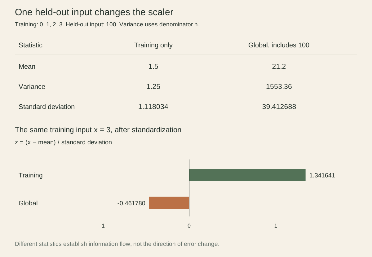
Take training inputs 0, 1, 2 and 3, with a held-out input of 100. The training mean is 1.5 and the variance, using the average squared deviation, is 1.25. Including 100 changes the mean to 21.2 and the variance to 1553.36.
The StandardScaler documentation describes storing training means and scales and uses the variance convention with denominator equal to the number of observed values. We use that convention here. This is not an assertion that every statistical variance estimator uses the same denominator.
Run the blocks in order in one Python interpreter. The fixture has nonempty finite rational inputs and strictly positive scale variances.
from fractions import Fraction as F
from math import sqrt


def moments(values):
    mean = sum(values) / len(values)
    variance = sum((x - mean)**2 for x in values) / len(values)
    return mean, variance


train_x = list(map(F, [0, 1, 2, 3]))
train_y = train_x.copy()
held_x = F(100)
train_mean, train_variance = moments(train_x)
global_mean, global_variance = moments(train_x + [held_x])
for name, mean, variance in [
    ('training', train_mean, train_variance),
    ('global', global_mean, global_variance),
]:
    z3 = float(F(3) - mean) / sqrt(float(variance))
    print(name, str(mean), str(variance), f'{z3:.6f}')
training 3/2 5/4 1.341641
global 106/5 38834/25 -0.461780The final number is the standardized value of training input 3. Under the training scaler it is above the fitted mean; under the global scaler it is below that mean. The held-out input has changed the representation used for training, despite its label never appearing in the calculation.
That observation proves information flow, but not a universal direction of performance change. Some estimators absorb particular coordinate changes. Others change their effective regularization or distance geometry. A trustworthy diagnosis distinguishes those cases instead of claiming that every leaked scaler necessarily improves a reported score.
A free intercept absorbs centering, but a penalty can preserve the scale effect
Give the four training inputs targets equal to their inputs. Consider a straight line fitted to standardized input z, with a free intercept and a penalty on its slope. The objective is average training squared error plus the penalty coefficient times the squared standardized slope. The intercept is not penalized.
Write the same prediction in raw input units as an intercept plus a raw slope times x. If the scaler variance is s², the squared standardized slope is s² times the squared raw slope. The scaling therefore changes the penalty on the raw function. With a free intercept, shifting the scaler’s mean can be absorbed into that intercept; it is the changed variance that matters in this example.
Minimizing the raw-coordinate objective gives:
raw slope = training covariance(x,y) / (training variance(x) + penalty*s²)
raw intercept = mean(training y) - raw slope*mean(training x)
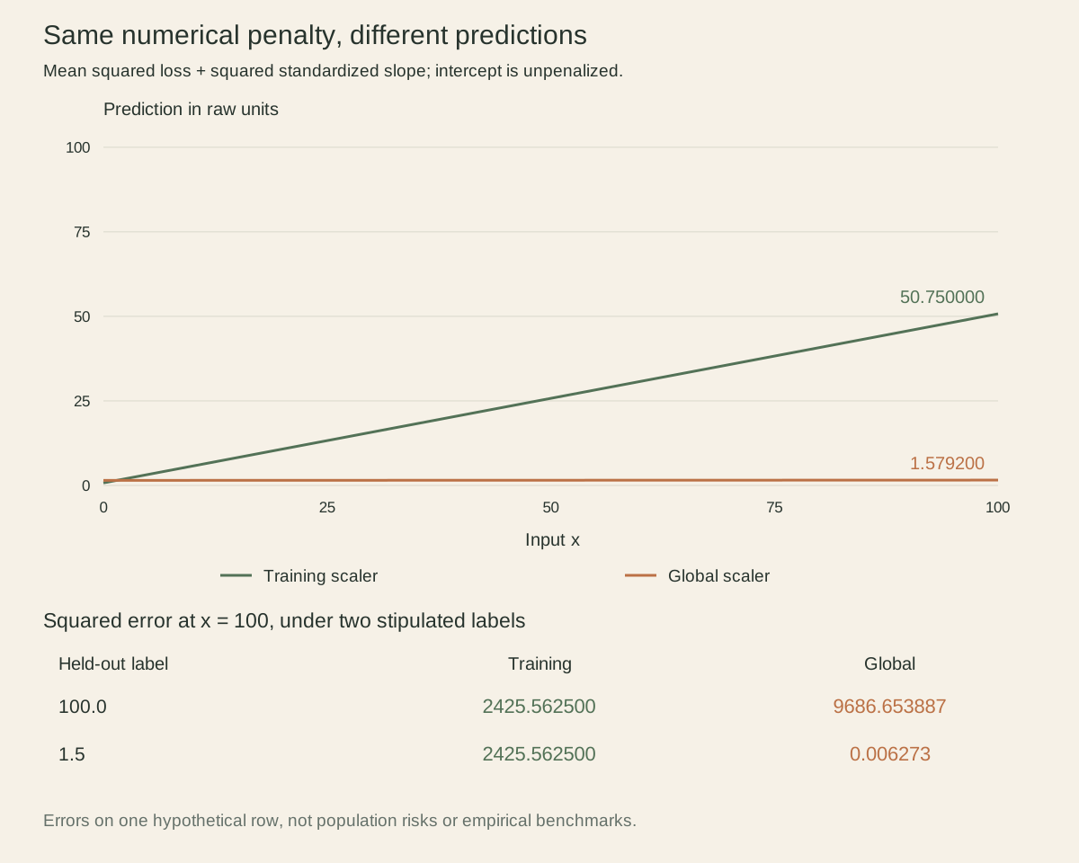
For these targets, the training covariance equals the training variance. A penalty of one with the training scaler yields slope one half and intercept three quarters. Using the global scaler with that same numerical penalty yields a slope of only about 0.000804. The held-out input has effectively imposed a much stronger penalty on variation in the raw prediction.
The next helper computes those exact coefficients. It assumes equal-length, nonempty finite rational training lists, a positive scale variance and a nonnegative penalty, with positive training variance for the unpenalized case. It is a small mathematical example, not a general input-validation library. Its objective uses mean loss; do not substitute a library’s sum-loss penalty parameter without checking the normalization.
def fit_scaled_ridge(x, y, scale_variance, penalty):
    mean_x, variance_x = moments(x)
    mean_y = sum(y) / len(y)
    covariance = sum((a-mean_x)*(b-mean_y) for a, b in zip(x, y)) / len(x)
    slope = covariance / (variance_x + penalty*scale_variance)
    return mean_y - slope*mean_x, slope


for name, scale_variance in [('training', train_variance), ('global', global_variance)]:
    intercept, slope = fit_scaled_ridge(train_x, train_y, scale_variance, F(1))
    prediction = intercept + slope*held_x
    errors = [(label-prediction)**2 for label in [F(100), F(3, 2)]]
    print(name, str(slope), f'{float(prediction):.6f}',
          *(f'{float(error):.6f}' for error in errors))

adjusted = train_variance / global_variance
assert fit_scaled_ridge(train_x, train_y, global_variance, adjusted) == (F(3,4), F(1,2))
for scale_variance in [train_variance, global_variance]:
    assert fit_scaled_ridge(train_x, train_y, scale_variance, F(0)) == (F(0), F(1))
print('adjusted penalty', str(adjusted))
training 1/2 50.750000 2425.562500 2425.562500
global 125/155461 1.579200 9686.653887 0.006273
adjusted penalty 125/155336After the name and exact slope, the columns are prediction at 100, squared error if the held-out label is 100, and squared error if that label is 1.5. The decimals are rounded displays of rational calculations.
Leakage can make this held-out error worse or better
With the training scaler, the prediction at 100 is 50.75. With the global scaler, it is about 1.5792. If the unseen label is 100, the global version has a much larger error. If the unseen label is 1.5, the global version has a much smaller error. Both are stipulated possible labels for the same input; neither label entered the fit.
These two worlds do not measure population risk or the frequency of either outcome. They establish that a leaked unsupervised transformation need not move every realized validation score in the same direction. The methodological problem is that the fitted procedure used information outside the intended boundary. A disappointing leaked score does not make the protocol valid, just as an attractive score does not prove a useful improvement.
For ordinary least squares with a free intercept and no penalty, either scaler produces raw slope one and intercept zero. Both predict 100 at the held-out input. An invertible affine transformation has merely rewritten the same class of lines. That invariance explains why a leakage check based only on whether predictions changed can miss an incorrect fitting boundary.
We can also restore the original ridge coefficients by reducing the global numerical penalty so its product with the global scale variance matches the training-only product. The asserted adjusted value in the program does exactly that. This is an explanation of coordinate dependence, not a recommendation to estimate a global scaler and compensate afterward. Arbitrary feature selection, imputations and nonlinear transforms do not share this simple cancellation.
Repeat the whole fitting boundary for every fold
For each cross-validation fold, start with an unfitted copy of the complete procedure. Fit its imputer, scaler and estimator on that fold’s training rows. Use their stored state to transform and predict that fold’s validation rows. Each fold may have different means, scales or selected features; that variation belongs to the learning procedure being evaluated.
The pipeline composition guide explains how pipelines fit transformers and predictors on the same training samples during cross-validation. It also documents caching fitted transformations when both the inputs and parameters match. A separately cached global scaler is not interchangeable with those fold-specific states. A custom cache must include the relevant training data identity and configuration, not just a filename such as scaled-data.
The held-out feature values still enter the prediction calculation. That is expected: predicting an input requires seeing it. What must remain fixed is the state learned from the training subset. For a direct boundary test, replace the held-out value while keeping the training subset constant and confirm that the stored training statistics remain unchanged. Predictions may change because the requested input changed; that is not evidence of leakage.
A pipeline cannot repair every source of information leakage
Feature selection based on correlations with all labels uses held-out targets to choose the representation. Place that selection inside each training fold. Do not first select one convenient common feature set using the full labeled dataset and then describe the later classifier cross-validation as untouched evaluation.
Group and time constraints also remain necessary. If recordings from one speaker appear on both sides, a correctly fitted scaler does not establish performance on new speakers. A historical feature built with a later label or a future aggregate remains unavailable at the original prediction time. A pipeline applies the inputs it receives; it does not prove how upstream features were produced.
A supervised transformer can also require separation inside its own training algorithm. For example, directly replacing a unique category with that row’s observed target reveals the answer to the downstream estimator. The outer fold boundary alone does not make such training features representative of what future predictions will receive. Specify the encoder’s internal handling of training targets and unseen categories instead of assuming that wrapping it in a pipeline is sufficient.
Missing and constant features need explicit behavior. The fixture avoids them so that every displayed division is defined. In an application, test a feature that is entirely missing in the training fold, a zero-variance feature and a category observed only in validation. Check the chosen transformer contract and resulting schema; do not fill gaps by computing statistics on the validation rows.
Exercises and a reproducible release check
First, replace the held-out input 100 with 10. The correctly fitted scaler still has mean 1.5 and variance 1.25; only its transformed query changes. The global scaler changes to mean 3.2 and variance 12.56. Recompute both ridge predictions and identify which operation was allowed to see the new value.
Next, multiply every input, including future queries, by ten. Transform the stored mean and variance consistently and verify that the standardized values and predictions stay the same. Contrast that coordinated unit change with inserting an additional held-out observation into the scaler fit. The two operations alter the computation for different reasons.
Finally, set the penalty to zero and verify that both fitted scalers give the same predictions while still storing different statistics. This exercise checks the information boundary directly rather than using a numerical prediction difference as its only signal.
Persist the evaluated transformation and estimator together, including feature order, missing-value behavior and category mappings. Apply that same state at inference. Record the split definition and the rows or data snapshot that fitted each state. A correct offline fold does not protect a deployment that independently recomputes a different scaler from incoming traffic.