Feature scaling changes the geometry of gradient descent
Derive how feature units change loss curvature, preserve a penalty when rescaling, and show why unit variance can leave a condition number of 100.
Feature scaling changes which parameter movements a gradient step treats as equally large. That can improve optimization when one input’s units create much greater curvature than another’s. It can also change the fitted model if coefficient penalties are left unchanged.
If you know linear regression and gradient descent, this foundation lesson separates those two effects using four invented observations. We derive a badly conditioned loss directly from the design matrix, repair its unit imbalance, then construct equally standardized features whose correlation leaves the condition number at 100. These are exact calculations, not measured training-speed comparisons.
Derive the geometry from four rows
Let the centered feature vectors be q = (-1,-1,1,1) and z = (-1,1,-1,1). Their mean squares are one and their mean product is zero. Use q as the first input and 10z as the second. With zero targets, no fitted intercept and the mean squared loss convention below, the coefficient loss is:
L(beta) = ||X beta||² / (2n), n = 4
H = XᵀX / n = diag(1,100)
L(beta) = (beta_1² + 100 beta_2²) / 2
For a symmetric positive-definite Hessian, the spectral condition number is its largest eigenvalue divided by its smallest: 100 here. We are discussing this specific matrix and Euclidean gradient descent, not a condition number independent of coordinates. Deep Learning’s numerical-computation chapter relates Hessian directional curvature to suitable step sizes.
At learning rate 0.019, the first coefficient is multiplied by 0.981 each update; the second by −0.9. From (1,1), after 100 updates their magnitudes are about 0.147 and 0.0000266. Both converge, but the shallow direction progresses slowly. Raising the rate to 0.02 reaches the nonconvergent boundary for a nonzero second component.
Run the three Python blocks sequentially. Fractions keep the design and update identities exact; the printed decimals merely summarize those values.
from fractions import Fraction as Q

q = tuple(map(Q, (-1, -1, 1, 1)))
z = tuple(map(Q, (-1, 1, -1, 1)))


def gram(rows):
    return tuple(tuple(sum(row[i]*row[j] for row in rows) / len(rows)
                       for j in range(2)) for i in range(2))


def mv(matrix, vector):
    return tuple(sum(a*b for a, b in zip(row, vector)) for row in matrix)


raw_rows = tuple(zip(q, (10*v for v in z)))
H = gram(raw_rows)
assert H == ((1, 0), (0, 100))
beta = (Q(1), Q(1))
eta = Q(19, 1000)
for _ in range(100):
    gradient = mv(H, beta)
    beta = tuple(b - eta*g for b, g in zip(beta, gradient))
assert beta == (Q(981, 1000)**100, Q(-9, 10)**100)
print(tuple(float(abs(b)) for b in beta))

scaled_H = gram(tuple(zip(q, z)))
theta = (Q(1), Q(10))
assert scaled_H == ((1, 0), (0, 1))
theta = tuple(t - g for t, g in zip(theta, mv(scaled_H, theta)))
assert theta == (0, 0)
Preserve predictions while changing coordinates
Divide the second input by ten and define theta_2 = 10 beta_2; keep theta_1 = beta_1. Every prediction is preserved because 10z beta_2 = z theta_2. The loss in the new coordinates is (theta_1² + theta_2²)/2, with identity Hessian. A rate-one step reaches the minimum exactly for this quadratic. The initial transformed coefficients are (1,10), representing the same starting predictions as the original (1,1).
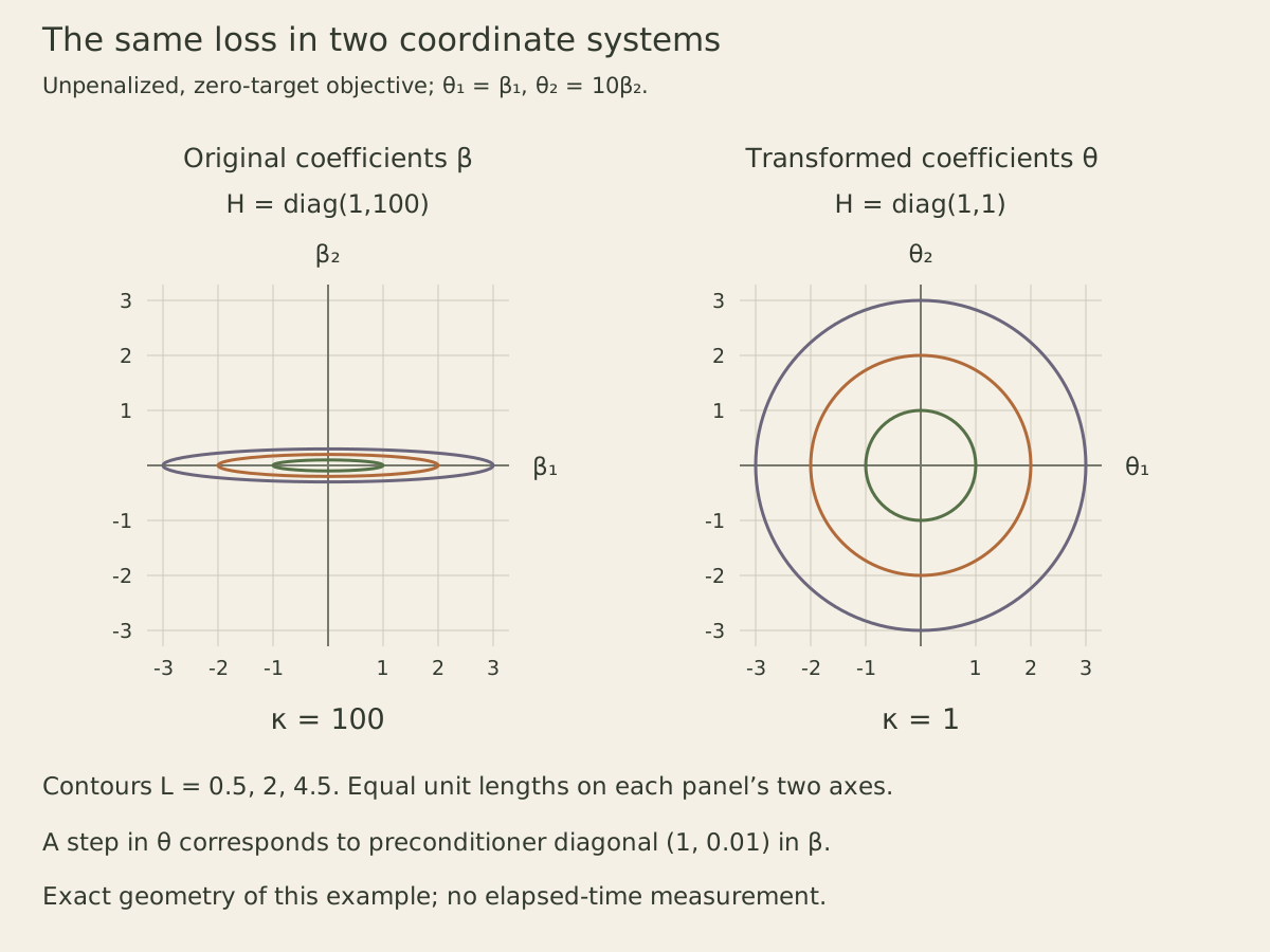
The contour levels agree across panels; the coordinates differ. In the original coordinates, the transformed update is a preconditioned step: multiply the original gradient’s second component by 0.01 before applying the common rate. It is a different optimization trajectory, not an identical update that happens to execute faster.
More generally, write theta = D beta and X_scaled = X D⁻¹ for an invertible diagonal scale matrix. The transformed Hessian is D⁻¹ H D⁻¹, and gradient descent there corresponds to beta_next = beta - eta D⁻² gradient_beta. These expressions assume real diagonal scales and the same scalar objective under the coordinate change. They do not describe arbitrary normalization layers.
An unchanged penalty can change the answer
Now change the target vector to 10z and add a coefficient penalty with strength one. In the original coordinates, the relevant part of the objective is 50(beta_2-1)² + beta_2²/2; the first coefficient optimizes to zero. Setting the derivative to zero gives beta_2 = 100/101.
After scaling the input, preserving that objective requires the penalty on the second transformed coefficient to be theta_2²/200. Keeping the apparently familiar penalty theta_2²/2 instead is a different modeling choice. Its optimum is five, corresponding to original coefficient 0.5 rather than 100/101.
raw_beta = Q(100, 101)
unchanged_penalty_theta = Q(5)
equivalent_penalty_theta = Q(1000, 101)
assert 100*(raw_beta - 1) + raw_beta == 0
assert (unchanged_penalty_theta - 10) + unchanged_penalty_theta == 0
assert (equivalent_penalty_theta - 10) + equivalent_penalty_theta/100 == 0
assert equivalent_penalty_theta/10 == raw_beta
assert unchanged_penalty_theta/10 == Q(1, 2)
print('Original coefficient:', raw_beta)
print('Same penalty after scaling:', unchanged_penalty_theta/10)
print('Transformed penalty:', equivalent_penalty_theta/10)
The discrepancy remains even if every optimizer reaches its exact minimum. It therefore cannot be explained by a faster solver or an insufficient iteration budget. Decide whether the experiment is about a coordinate change preserving the objective or a different penalty expressed in standardized units. Both can be useful, but they answer different questions.
This example defines its own mean-loss and penalty factors explicitly. A library’s alpha need not use that same normalization. Translate its documented objective before transferring the numeric value one into an API call.
Unit variance does not remove correlation
For the next calculation, return to the unpenalized, zero-target loss.
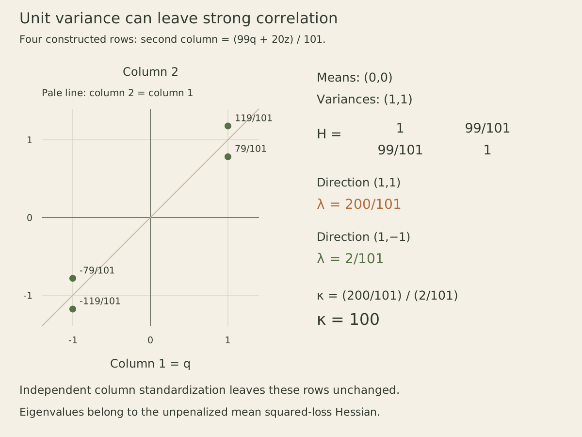
StandardScaler’s documentation defines independent centering and scaling of each feature and uses the variance convention with divisor n. Consider a new second column (99q + 20z)/101. It already has mean zero and variance one because 99² + 20² = 101². Its correlation with q is nevertheless 99/101.
rho = Q(99, 101)
mix = Q(20, 101)
correlated_rows = tuple((a, rho*a + mix*b) for a, b in zip(q, z))
assert all(sum(row[j] for row in correlated_rows) == 0 for j in range(2))
correlated_H = gram(correlated_rows)
assert correlated_H == ((1, rho), (rho, 1))
assert mv(correlated_H, (1, 1)) == (1 + rho, 1 + rho)
assert mv(correlated_H, (1, -1)) == (1 - rho, -(1 - rho))
assert (1 + rho)/(1 - rho) == 100
print('Curvatures:', 1 + rho, 1 - rho)
print('Condition number:', (1 + rho)/(1 - rho))

inverse_H = ((1/(1-rho*rho), -rho/(1-rho*rho)),
             (-rho/(1-rho*rho), 1/(1-rho*rho)))
beta = (Q(2), Q(-3))
assert mv(inverse_H, mv(correlated_H, beta)) == beta
The directions (1,1) and (1,-1) have eigenvalues 200/101 and 2/101. Their curvature ratio is still 100. Standardizing each column again does nothing to this exact dataset. The short final assertion shows what an exact full-matrix preconditioner would accomplish for this positive-definite quadratic: it turns the gradient into the displacement from the zero-target optimum.
Scikit-learn’s preprocessing guide distinguishes feature-wise scaling from whitening, which can remove linear correlations. A full covariance or curvature transformation requires estimating and applying more than separate column scales. Explicitly forming an inverse is unnecessary in a practical solver; a suitable linear solve or factorization is usually preferable. The exact inverse above explains the geometry rather than prescribing a production implementation.
At perfect duplication, the second feature equals q and the Hessian is singular. Coefficients (1,0) and (0,1) give identical predictions on all four rows. No invertible rescaling creates the missing independent direction or makes those coefficients uniquely identifiable from this design. A zero-variance column also cannot become informative merely by dividing by a scale. The scaler documentation describes a scale factor of one for zero variance; that convention does not repair rank.
Compare equivalent problems deliberately
For a scaling experiment, retain the same data split, loss definition and initial predictions. If preserving the statistical objective, transform its penalty too. Record iteration counts separately from elapsed time: the one-step identity in this lesson is not a wall-clock benchmark. Compare loss or predictions in a common representation, since raw gradient norms and coefficient-update sizes change with the coordinate units.
In the first unpenalized example, the initial raw gradient is (1,100) while the transformed gradient is (1,10). Their squared Euclidean norms are 10,001 and 101 even before either optimizer moves. A smaller gradient norm after scaling therefore need not mean a better prediction or a lower objective. A stopping rule expressed in coefficient-gradient units must account for the transformation; otherwise one run can stop earlier simply because its numerical coordinates changed.
Estimate scales only from the training portion, then reuse those values on validation and later inputs. The preprocessing guide describes this train-and-transform separation. Outliers can dominate ordinary variance estimates; changing to a robust scale changes the transformation being evaluated. For other losses, the Hessian may depend on predictions and additional weights, so unit feature variance need not imply equal loss curvature even without strong linear correlation.
For an exercise, multiply the second raw feature by 100 instead of ten. Its unpenalized Hessian entry becomes 10,000; preserving predictions requires theta_2 = 100 beta_2, and preserving a unit original coefficient penalty requires transformed strength 1/10000 in that direction. Next replace 99/101 and 20/101 with 3/5 and 4/5. Derive unit variances, correlation 3/5 and condition number four. Finally set the second feature equal to the first and identify which coefficient sums remain observable. These checks distinguish poor units, near redundancy and actual loss of rank.